Pre-Training Large Language Models with FP8: A Comprehensive Benchmark on NVIDIA B200 GPUs
A comprehensive guide to FP8 (8-bit floating point) training for large language models, exploring performance benefits and implementation strategies on NVIDIA B200 GPUs
deep-learning
fp8
low-precision
pytorch
optimization
Author
Dipankar Baisya
Published
December 30, 2025
1 Introduction
As large language models continue to grow in size and complexity, pre-training them efficiently has become a critical challenge for researchers and practitioners. Traditional training with 32-bit (FP32) or even 16-bit (BF16) precision requires substantial computational resources and memory. Low-precision training, particularly with 8-bit floating point (FP8) format, has emerged as a promising solution to reduce both memory footprint and training time while maintaining model quality.
This blog post presents a comprehensive exploration of FP8 training, from theoretical foundations to practical implementation, culminating in detailed benchmark results comparing FP8 and BF16 training across multiple model architectures on NVIDIA’s latest B200 (Blackwell) GPUs. We’ll walk through the implementation using PyTorch’s torchao library and HuggingFace Accelerate, and analyze empirical findings that reveal when and why FP8 training excels.
2 Understanding Low-Precision Training
2.1 What is Low-Precision Training?
Low-precision training refers to using reduced numerical precision (fewer bits) for representing numbers during neural network training. Instead of standard 32-bit floating point (FP32), models can be trained using 16-bit (FP16/BF16) or even 8-bit (FP8) formats. The key insight is that compute happens in low precision, but results are upcast and accumulated in higher precision to maintain numerical stability.
2.2 Comparison of Low-Precision Methods
According to HuggingFace Accelerate documentation, different low-precision training methods offer varying trade-offs between memory usage, computation speed, and accuracy. Here’s a comprehensive comparison:
Optimization Level
Computation (GEMM)
Comm
Weight
Master Weight
Weight Gradient
Optimizer States
FP16 AMP
FP16
FP32
FP32
N/A
FP32
FP32+FP32
Nvidia TE
FP8
FP32
FP32
N/A
FP32
FP32+FP32
MS-AMP O1
FP8
FP8
FP16
N/A
FP8
FP32+FP32
MS-AMP O2
FP8
FP8
FP16
N/A
FP8
FP8+FP16
MS-AMP O3
FP8
FP8
FP8
FP16
FP8
FP8+FP16
Key observations:
FP16 AMP (Automatic Mixed Precision): The baseline mixed-precision approach, computing in FP16 while keeping weights and optimizer states in FP32
Nvidia TransformersEngine (TE): Converts matrix multiplications to FP8 while keeping other operations in FP32, providing maximum stability with minimal accuracy loss
MS-AMP O1: Extends FP8 to communication operations, reducing distributed training bandwidth by ~50%
MS-AMP O2: Further reduces optimizer states to mixed FP8/FP16, balancing memory savings and numerical stability
MS-AMP O3: Most aggressive approach with full FP8 except FP16 master weights, maximizing memory reduction
2.3 The Core Principle: Compute vs Storage
The fundamental principle of low-precision training is:
✅ Fast computation in low precision (FP8/FP16) on modern GPU tensor cores
✅ Numerical stability by accumulating in high precision (BF16/FP32)
✅ Memory savings during computation (parameters and activations)
✅ Training stability maintained across many gradient updates
Example: FP8 Forward Pass
1. Parameters stored in BF16
2. Cast weights and activations to FP8
3. Matrix multiplication: FP8 × FP8 (fast!)
4. Upcast result to BF16
5. Store activations in BF16 for backward pass
This prevents accumulation errors that would occur if all operations remained in FP8, while still gaining the computational speedup from low-precision arithmetic.
3 Float8 (FP8) Format: Technical Deep Dive
3.1 What is FP8?
Float8 (FP8) is an 8-bit floating-point format that represents numbers using only 8 bits, compared to 32 bits for FP32 or 16 bits for FP16/BF16. According to the PyTorch blog on FP8 training, FP8 provides a crucial balance between memory efficiency and computational precision for large-scale training.
3.2 FP8 Format Structure
FP8 typically uses the following bit allocation:
1 sign bit: Positive or negative
4-5 exponent bits: Determines the range of representable values
2-3 mantissa bits: Determines precision within that range
Precision Comparison Table:
Precision
Total Bits
Exponent
Mantissa
Range
Precision
Use Case
FP32
32
8 bits
23 bits
±3.4e38
~7 decimal digits
Master weights, accumulation
BF16
16
8 bits
7 bits
±3.4e38
~3 decimal digits
Training (good range)
FP16
16
5 bits
10 bits
±65,504
~3 decimal digits
Training (limited range)
FP8
8
4-5 bits
2-3 bits
±57,344
~2 decimal digits
Computation only
3.3 Key Characteristics
Memory Efficiency:
75% reduction compared to FP32
50% reduction compared to FP16/BF16
Critical for training billion-parameter models
Computational Performance:
2x faster matrix multiplications vs BF16
4x faster vs FP32
Leverages modern GPU tensor cores (NVIDIA H100, B200)
Precision Trade-off:
Limited precision (~2 significant decimal digits)
Requires dynamic scaling to maximize representable range
Must upcast for accumulation to avoid compounding errors
This ensures values use the full FP8 range, minimizing quantization errors.
3.6 Detailed FP8 Training Flow with FSDP2
Let’s examine the complete precision management flow in FP8 training with FSDP2, as implemented in our benchmark.
3.6.1 Forward Pass Flow
┌─────────────────────────────────────────────────────────────┐
│ Step 1: Parameter Storage (BF16, sharded across GPUs)      │
│         • Each GPU stores 1/N of model parameters           │
│         • Base dtype: BF16 (16 bits per parameter)          │
└─────────────────────────────────────────────────────────────┘
                            ↓
┌─────────────────────────────────────────────────────────────┐
│ Step 2: All-Gather in FP8 (FSDP2 communication)            │
│         • Parameters gathered from all GPUs in FP8          │
│         • Saves 2x bandwidth vs BF16                        │
│         • enable_fsdp_float8_all_gather=True                │
│         • 8 bits/param vs 16 bits/param                     │
└─────────────────────────────────────────────────────────────┘
                            ↓
┌─────────────────────────────────────────────────────────────┐
│ Step 3: Upcast FP8 → BF16                                   │
│         • Parameters converted to BF16 after gathering      │
│         • Ensures numerical stability for computation       │
└─────────────────────────────────────────────────────────────┘
                            ↓
┌─────────────────────────────────────────────────────────────┐
│ Step 4: Matrix Multiply in FP8                              │
│         • Weights: BF16 → FP8 (cast to 8-bit)               │
│         • Activations: BF16 → FP8 (cast to 8-bit)           │
│         • Computation: FP8 × FP8 (fast tensor cores!)       │
│         • 2x speedup vs BF16 × BF16                         │
└─────────────────────────────────────────────────────────────┘
                            ↓
┌─────────────────────────────────────────────────────────────┐
│ Step 5: Upcast Results FP8 → BF16                           │
│         • Critical for numerical stability                  │
│         • Prevents accumulation errors                      │
│         • Result has full BF16 precision                    │
└─────────────────────────────────────────────────────────────┘
                            ↓
┌─────────────────────────────────────────────────────────────┐
│ Step 6: Store Activations (BF16)                            │
│         • Needed for backward pass                          │
│         • Higher precision for gradient computation         │
└─────────────────────────────────────────────────────────────┘
3.6.2 Backward Pass Flow
┌─────────────────────────────────────────────────────────────┐
│ Step 1: Compute Gradients in BF16                           │
│         • Uses stored BF16 activations                      │
│         • Chain rule applied in higher precision            │
└─────────────────────────────────────────────────────────────┘
                            ↓
┌─────────────────────────────────────────────────────────────┐
│ Step 2: Cast Gradients BF16 → FP8                           │
│         • For storage and communication                     │
│         • Reduces memory footprint by 2x                    │
└─────────────────────────────────────────────────────────────┘
                            ↓
┌─────────────────────────────────────────────────────────────┐
│ Step 3: Reduce-Scatter in FP8                               │
│         • Gradients averaged across GPUs                    │
│         • Communicated in FP8 (saves bandwidth)             │
│         • Each GPU receives its gradient shard              │
└─────────────────────────────────────────────────────────────┘
                            ↓
┌─────────────────────────────────────────────────────────────┐
│ Step 4: Upcast to BF16 for Optimizer                        │
│         • Optimizer needs higher precision                  │
│         • Ensures stable parameter updates                  │
└─────────────────────────────────────────────────────────────┘
                            ↓
┌─────────────────────────────────────────────────────────────┐
│ Step 5: Update Parameters (BF16)                            │
│         • AdamW updates master weights in BF16              │
│         • Maintains numerical stability over many steps     │
└─────────────────────────────────────────────────────────────┘
3.7 The Accumulation Problem: Why Upcasting is Essential
The core challenge: FP8 has very limited precision (~3-4 significant decimal digits). When you accumulate many small values, errors compound catastrophically.
Example: Accumulation in FP8 (Bad!)
# Simulated FP8 accumulation - DO NOT DO THIS!result = fp8(0.0)for i inrange(1000): small_value = fp8(0.001) result += small_value # Each addition loses precision!# Expected result: 1.0# Actual result: 0.87 or worse (accumulated rounding errors)# Error: ~13% due to precision loss at each step
Why this fails:
Each FP8 addition introduces ~0.0001-0.001 rounding error
1000 additions → errors accumulate
Final result is significantly wrong
Solution: Compute in FP8, Accumulate in BF16 (Good!)
# Correct approach: upcast before accumulatingresult = bf16(0.0)for i inrange(1000): small_value = fp8(0.001) # Compute in FP8 result += bf16(small_value) # Upcast before accumulating# Expected result: 1.0# Actual result: 0.999 (accurate!)# Error: ~0.1% - acceptable for training
Why this works:
BF16’s 7-bit mantissa preserves precision during accumulation
Only the initial computation uses FP8 (fast)
Accumulation uses BF16 (stable)
Best of both worlds: speed + stability
Real training example:
Consider a gradient update in a transformer:
# Wrong: accumulate gradients in FP8for layer in model.layers: grad_fp8 = compute_gradient_fp8(layer) total_grad_fp8 += grad_fp8 # Error accumulates!# Right: accumulate gradients in BF16for layer in model.layers: grad_fp8 = compute_gradient_fp8(layer) total_grad_bf16 += grad_fp8.to(bf16) # Stable accumulation
3.8 Operation-Level Precision Strategy
Different operations in neural network training have different precision requirements. Here’s the optimal strategy used in our benchmark:
Operation
Precision
Rationale
Impact
Matrix Multiply
FP8
Bulk of computation; 2-4x speedup on modern GPUs
60-80% of training time
Activation Functions
BF16
Non-linear ops benefit from higher precision
Small overhead, better accuracy
Result Accumulation
BF16
Prevents compounding rounding errors
Critical for stability
Gradient Computation
BF16
Maintains gradient accuracy for backprop
Essential for convergence
Parameter Updates
BF16/FP32
Critical for long-term training stability
Optimizer needs precision
Communication (FSDP)
FP8
Reduces network bandwidth by 2x
Speeds up multi-GPU training
Parameter Storage
BF16
Master weights for optimizer
Memory vs precision balance
Normalization (LayerNorm)
BF16
Statistics computation needs precision
Prevents numerical instability
Residual Connections
BF16
Direct addition benefits from precision
Maintains gradient flow
Performance impact breakdown:
For a Llama 3.1 8B model:
Matrix multiplications: ~75% of FLOPs → FP8 gives 2x speedup here
Other operations: ~25% of FLOPs → Stay in BF16 for stability
This explains why we see 10-15% TFLOPs improvement rather than 2x in our benchmarks.
3.9 Traditional Mixed Precision Training (FP16/BF16) - Historical Context
Before FP8, the standard was FP16/BF16 mixed precision training:
Flow:
1. Master Weights: Stored in FP32 (high precision)
   ↓
2. Cast to FP16/BF16 for forward pass
   ↓
3. Compute: Matrix multiplications in FP16/BF16 (2x faster than FP32)
   ↓
4. Activations: Stored in FP16/BF16 (50% memory vs FP32)
   ↓
5. Backward Pass: Gradients computed in FP16/BF16
   ↓
6. Upcast: Gradients converted to FP32 before optimizer
   ↓
7. Optimizer: Updates master weights in FP32
Key insight: Even with FP16 computation, optimizer maintains FP32 master copy to prevent precision loss over thousands of gradient updates.
FP8 extends this principle:
Compute: FP8 (even lower precision, 2x faster than BF16)
Accumulate: BF16 (sufficient precision for stability)
Master weights: BF16 (good enough for billion-parameter models)
This hierarchical precision strategy is the foundation of modern efficient training.
4 TorchAO’s convert_to_float8_training: Enabling FP8 at Scale
4.1 Overview
The torchao library provides convert_to_float8_training, a function that seamlessly converts torch.nn.Linear modules to FP8-enabled Float8Linear modules for efficient training.
4.2 Basic Usage
from torchao.float8 import convert_to_float8_training, Float8LinearConfigimport torchimport torch.nn as nn# Create modelmodel = nn.Sequential( nn.Linear(8192, 4096, bias=False), nn.Linear(4096, 128, bias=False),).bfloat16().cuda()# Configure FP8 recipeconfig = Float8LinearConfig.from_recipe_name("tensorwise")# Convert eligible linear modules to FP8convert_to_float8_training(model, config=config)# Enable torch.compile for best performancemodel = torch.compile(model)
4.3 Configuration Recipes
TorchAO provides three FP8 recipes with different speed/accuracy trade-offs:
1. “tensorwise” - Fastest but least accurate
Scales entire tensors by a single factor
Minimal overhead
Best for throughput-critical applications
2. “rowwise” - Balanced performance and accuracy
Scales each row independently
Better numerical properties
Recommended for most use cases
3. “rowwise_with_gw_hp” - Most accurate
Row-wise scaling with high-precision gradients
Maintains gradient accuracy
Best for quality-critical training
4.4 Optional Module Filtering
You can selectively convert modules using a filter function:
def module_filter_fn(mod: torch.nn.Module, fqn: str):# Skip first and last layers (common practice)if fqn in ["0", "model.layers.-1"]:returnFalse# Only convert layers with dimensions divisible by 16ifisinstance(mod, torch.nn.Linear):if mod.in_features %16!=0or mod.out_features %16!=0:returnFalsereturnTrueconvert_to_float8_training( model, config=config, module_filter_fn=module_filter_fn)
Why skip first/last layers?
Input embeddings and output layers are often more sensitive to precision
Keeping them in higher precision improves model quality with minimal cost
4.5 Performance Impact
According to torchao benchmarks on NVIDIA H100 with 8 GPUs:
Tensorwise scaling: ~25% speedup over BF16 baseline
Rowwise scaling: ~10% speedup with better accuracy
E2E training speedups: Up to 1.5x at 512 GPU / 405B parameter scale
HuggingFace provides a reference implementation showing how to use FP8 with DistributedDataParallel (DDP).
5.2 Implementation Walkthrough
Step 1: Identify Linear Layers
def train_baseline(): set_seed(42) model, optimizer, train_dataloader, eval_dataloader, lr_scheduler = get_training_utilities(MODEL_NAME)# Find first and last linear layers first_linear =None last_linear =Nonefor name, module in model.named_modules():ifisinstance(module, torch.nn.Linear):if first_linear isNone: first_linear = name last_linear = name
Why identify first/last layers? The first and last linear layers are typically excluded from FP8 conversion for numerical stability:
First layer: Processes input embeddings, which can have wide dynamic range
Last layer: Produces final logits for loss computation, where precision matters
The FP8 model is wrapped with PyTorch’s DistributedDataParallel for multi-GPU training.
Step 5: Training Loop with Autocast
for batch in train_dataloader:with torch.autocast(device_type="cuda", dtype=torch.bfloat16): outputs = model(**batch) loss = outputs.loss loss.backward() optimizer.step() optimizer.zero_grad()
Key points:
Autocast context: Ensures non-FP8 operations use BF16
DDP gradient synchronization: Gradients are all-reduced across GPUs automatically
Mixed precision: FP8 for linear layers, BF16 for other operations
5.3 DDP vs FSDP: When to Use Each
Use DDP when:
Model fits in single GPU memory
Simple multi-GPU setup needed
Maximum per-GPU throughput desired
Use FSDP when:
Model too large for single GPU
Need to scale to 100+ GPUs
Memory efficiency is critical
6 FP8 with FSDP2: Production-Scale Training
6.1 FSDP2 Overview
FSDP2 (Fully Sharded Data Parallel 2) is PyTorch’s latest distributed training framework that shards model parameters, gradients, and optimizer states across GPUs. This enables training models that wouldn’t fit on a single GPU.
The FSDP2 approach lets Accelerate manage the order of operations:
✅ Ensures FP8 conversion happens before FSDP wrapping
✅ Prevents user errors (wrong order of operations)
✅ Cleaner API (one call to prepare() does everything)
✅ Handles edge cases (e.g., certain layers shouldn’t be converted)
Verification:
You can verify this by inspecting the model after prepare():
model = AutoModelForCausalLM.from_config(...)print(type(model.model.layers[0].mlp.gate_proj))# Output: <class 'torch.nn.Linear'>model = accelerator.prepare(model) # With AORecipeKwargsprint(type(model.model.layers[0].mlp.gate_proj))# Output: <class 'torchao.float8.float8_linear.Float8Linear'># ↑ Linear layers converted to Float8Linear!
Each transformer decoder layer becomes a separate FSDP unit
Parameters are sharded at the layer level
Provides good balance between:
Communication efficiency (fewer all-gathers)
Memory efficiency (fine-grained sharding)
6.7 Why cpu_ram_efficient_loading=False?
cpu_ram_efficient_loading=False# Incompatible with FP8 torchao
CPU-efficient loading creates the model on CPU first, then transfers to GPU. This is incompatible with torchao’s FP8 conversion, which must happen on GPU. Setting this to False ensures the model is created directly on GPU.
7 Our Implementation: Code Highlights
Our benchmark implementation (fp8_benchmark.py) builds on these concepts to create a comprehensive FP8 vs BF16 comparison framework. Let’s examine key highlights from the codebase.
Why this matters: Different model architectures use different layer class names. FSDP2’s auto-wrap policy needs the correct class name to shard the model properly. Supporting multiple architectures allows comprehensive benchmarking across model families.
FSDP2 plugin configured for transformer-based wrapping
Mixed precision set to “fp8” or “bf16”
FP8 config enables optimized all-gather
Config passed to Accelerator via kwargs_handlers
7.3 Model Initialization Strategy
# Lines 124-127: Random initialization for benchmarkingmodel = AutoModelForCausalLM.from_config( AutoConfig.from_pretrained(args.model_name, use_cache=False), torch_dtype=torch.bfloat16,)
Key observation: We use from_config() instead of from_pretrained(), creating models with random weights. This is intentional for benchmarking:
✅ Advantages:
Much faster initialization (no weight loading)
Sufficient for performance testing
Loss values still meaningful for convergence comparison
❌ Not suitable for:
Fine-tuning tasks
Evaluating model quality
Production training
This is a pre-training benchmark, not actual pre-training. We run only 50-1000 steps to measure performance, not the billions of steps needed for real pre-training.
7.4 Performance Tracking
# Lines 143-157: Training loop with metricsfor step, batch inenumerate(dataloader): outputs = model(**batch) loss = outputs.loss accelerator.backward(loss) optimizer.step() optimizer.zero_grad()# Track performance metrics metrics = performance_tracker.step( batch["input_ids"].shape[1], model_flops_per_token )
Tracked metrics:
Tokens/second: Total tokens processed per second
Steps/second: Training iterations per second
TFLOPs: Teraflops (trillion floating-point operations per second)
MFU: Model FLOPs Utilization (% of theoretical peak)
GPU memory: Active, allocated, and reserved memory
7.5 Loss Function
# The loss is automatically computed inside the modeloutputs = model(**batch)loss = outputs.loss # Cross-entropy loss
When labels are provided to a HuggingFace causal language model, it automatically computes cross-entropy loss for next-token prediction:
This measures how well the model predicts the next token given previous context.
7.6 FSDP Communication Pattern
During training, FSDP2 follows this communication pattern:
Forward Pass:
1. All-gather parameters in FP8 (if enabled) or BF16
2. Upcast to BF16 after gathering
3. Compute forward pass
4. Free gathered parameters
5. Store activations for backward pass
Backward Pass:
1. All-gather parameters again
2. Compute gradients
3. Reduce-scatter gradients (average across GPUs)
4. Each GPU receives its gradient shard
5. Free gathered parameters
6. Update local parameter shard
This pattern enables training models larger than single-GPU memory while minimizing communication overhead through FP8 compression.
8 Experimental Setup: Benchmarking on NVIDIA B200
8.1 Hardware Configuration
Our experiments were conducted on a Lambda Cloud instance with:
Our benchmark results represent best-case FP8 performance with optimal hardware. If deploying on PCIe-based systems:
Expect 20-40% lower multi-GPU throughput than reported here
FP8’s communication bandwidth advantage becomes more critical
May need larger local batch sizes to amortize communication cost
Consider gradient accumulation to reduce synchronization frequency
Lambda Cloud Instance Specifications:
Instance type: GPU Cloud with 4× B200 SXM6
Network: NVLink Gen 5.0 (900 GB/s per GPU)
Host-to-GPU: PCIe Gen 5.0 (only for CPU-GPU transfers, not GPU-GPU)
Availability: Lambda Labs on-demand instances
8.2 NVIDIA B200 (Blackwell) Architecture
The B200 represents NVIDIA’s latest generation of data center GPUs:
Key features:
2nd generation Transformer Engine with FP8 support
Significantly higher FP8 throughput (9000 TFLOPs)
Larger memory capacity (180GB vs 80GB on H100)
Improved NVLink for multi-GPU scaling
Why B200 matters for FP8: The Blackwell architecture has hardware-optimized FP8 tensor cores, making it the ideal platform for evaluating FP8 training performance.
8.3 Software Stack
PyTorch: 2.0+
torchao: 0.1.0+ (FP8 support)
HuggingFace Transformers: 4.30.0+
HuggingFace Accelerate: 0.20.0+ (FSDP2 support)
CUDA: 12.1
8.4 Benchmark Configuration
Training Configuration:
Batch size: 1 per GPU (intentionally small to isolate effects)
Sequence lengths: 2048, 4096, 8192 tokens
GPU counts: 1, 2, 4 GPUs
Precision: FP8 vs BF16
Optimization: AdamW with fused implementation
Learning rate: 1e-5
Training steps: 50-1000 (depending on model/configuration)
Models Tested:
Llama 3.2 1B - Small efficient model
Llama 3.2 3B - Medium-sized model
Llama 3.1 8B - Large model
Qwen3 4B - Alternative architecture
Qwen3 14B - Very large model (4 GPUs only)
8.5 Dataset
TinyStories: A dataset of simple short stories
Used for pre-training benchmarks
Tokenized and packed into fixed-length sequences
First 10% of dataset used (~10,000 sequences)
8.6 Experimental Design
Goal: Compare FP8 vs BF16 across:
Performance metrics: TFLOPs, tokens/s, MFU
Training quality: Loss convergence
Scalability: 1, 2, 4 GPU configurations
Model sizes: 1B to 14B parameters
Sequence lengths: 2048 to 8192 tokens
Controlled variables:
Same random seed (42) for reproducibility
Same model architectures and hyperparameters
Same dataset and data preprocessing
Same optimizer and learning rate
Measured variables:
Computational throughput (TFLOPs)
Token processing throughput (tokens/s)
Hardware utilization (MFU %)
Training loss progression
GPU memory usage
8.7 Why Batch Size = 1?
We intentionally used batch_size=1 per GPU to:
✅ Isolate sequence length effects: Focus on how sequence length impacts performance without batch size confounding
✅ Reveal precision sensitivity: Smaller batches expose FP8’s precision limitations (as we’ll see in results)
✅ Test worst-case scenario: If FP8 works well at batch_size=1, it will excel at larger batches
❌ Not representative of production: Real training typically uses batch_size=4-8 per GPU for better efficiency
This design choice led to one of our most interesting findings: the dramatic difference between FP8 and BF16 on single GPU vs multi-GPU setups.
8.8 Important Note: Pre-Training Benchmark vs Production Pre-Training
This benchmark implements a pre-training setup (training from scratch with random initialization) rather than fine-tuning or inference. However, it’s crucial to understand that this is a benchmark for measuring performance, not actual production pre-training.
8.8.1 Evidence This is Pre-Training (Not Fine-Tuning)
Looking at our code (fp8_benchmark.py, lines 124-127):
model = AutoModelForCausalLM.from_config( AutoConfig.from_pretrained(args.model_name, use_cache=False), torch_dtype=torch.bfloat16,)
Key observation: We use from_config() instead of from_pretrained(), meaning:
✅ Model starts with random initialization (not pretrained weights)
✅ Trains from scratch on text corpus (TinyStories dataset)
✅ Uses cross-entropy loss for next-token prediction
✅ This is the definition of pre-training
If this were fine-tuning, we would see:
❌ from_pretrained() to load pretrained weights
❌ Task-specific dataset (not general text)
❌ Potentially different loss function or training objective
8.8.2 Evidence This is a Benchmark (Not Production Pre-Training)
However, several characteristics distinguish this from actual production pre-training:
Characteristic
This Benchmark
Production Pre-Training
Training steps
50-1000 steps
Billions of steps
Training duration
Minutes to hours
Weeks to months
Model initialization
Random weights
Random weights
Primary goal
Measure performance
Train useful model
Model saving
❌ Not saved
✅ Checkpoints saved
Dataset
TinyStories (simple)
Diverse web text, books
Metrics tracked
TFLOPs, tokens/s, MFU
Loss, perplexity, downstream task performance
Hardware scale
1-4 GPUs
100-1000s of GPUs
Total tokens
~10M tokens
Trillions of tokens
Cost
$10-100
Millions of dollars
8.8.3 Primary Use Case: Performance Benchmarking
The primary purpose of this code is to:
✅ Measure and compare FP8 vs BF16 training performance
Computational throughput (TFLOPs)
Token processing speed (tokens/s)
Hardware utilization (MFU %)
Training loss convergence patterns
Memory usage
✅ Quantify benefits of FP8 training
Speedup: ~10-15% TFLOPs improvement
Memory: 50% reduction for parameters/activations
Communication: 2x bandwidth reduction in FSDP
Quality: Identify when FP8 matches BF16 (multi-GPU) vs when it fails (single GPU)
✅ Guide infrastructure decisions
Should we use FP8 for our training job?
What’s the minimum GPU count for FP8?
What batch size do we need?
Which sequence length is most efficient?
8.8.4 Why Random Initialization is Sufficient for Benchmarking
Random initialization works for performance benchmarking because:
Computational patterns are identical: Random weights produce the same GEMM (matrix multiplication) operations as pretrained weights
Loss convergence is meaningful: Even random initialization shows clear convergence trends that reveal optimization dynamics
Much faster: No need to download/load multi-GB pretrained checkpoints
Reproducible: Fixed random seed ensures consistent results
What random initialization doesn’t show:
Final model quality on downstream tasks
Long-term training stability (1000s of steps)
Interactions with pretrained weight distributions
8.8.5 Production Pre-Training Would Require
To turn this into actual production pre-training, you would need:
# 1. Much longer trainingnum_steps =100_000_000# Billions instead of 50# 2. Larger, more diverse datasetfrom datasets import load_datasetdataset = load_dataset("c4", split="train") # Not TinyStories# 3. Save checkpointsif step %1000==0: accelerator.save_state(f"checkpoint-{step}")# 4. Track model quality metricseval_perplexity = evaluate_on_validation_set(model)accelerator.log({"perplexity": eval_perplexity})# 5. Much larger scalenum_gpus =256# Not just 1-4batch_size_per_gpu =4# Not just 1
8.8.6 Value of This Benchmark Approach
The benchmark approach (short runs with random initialization) provides invaluable insights without the time and cost of full pre-training:
Time savings:
Benchmark: Hours to complete full sweep
Production pre-training: Weeks to months
Cost savings:
Benchmark: $50-500 in GPU time
Production pre-training: $1M-100M in GPU time
Insights gained:
✅ Performance characteristics of FP8 vs BF16
✅ Optimal batch size and sequence length
✅ Multi-GPU scaling efficiency
✅ Hardware utilization (MFU)
✅ Critical finding: FP8 requires multi-GPU or larger batches
These insights inform actual production training decisions, allowing teams to optimize their multi-million dollar training jobs before committing resources.
9 Experimental Results and Analysis
Our comprehensive benchmark reveals nuanced performance characteristics of FP8 training across different configurations. Let’s examine each metric with detailed plots and analysis.
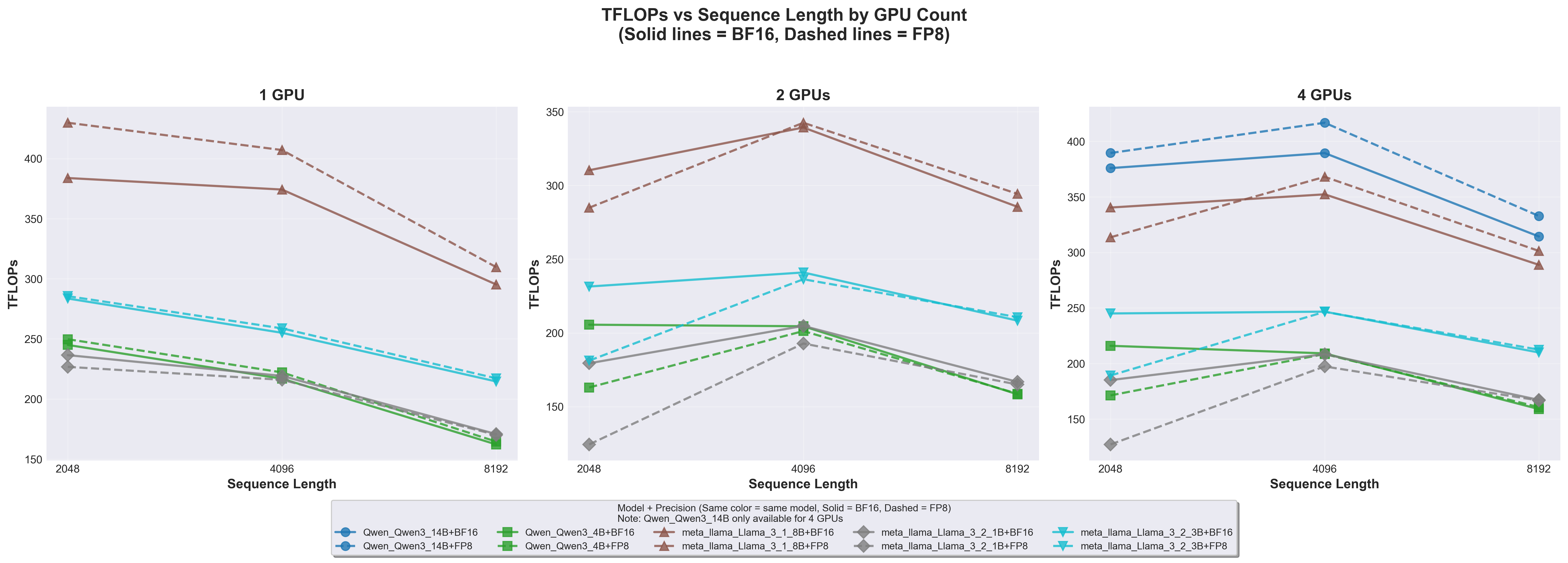
9.1 Computational Throughput: TFLOPs vs Sequence Length
TFLOPs vs Sequence Length
9.1.1 Key Findings
FP8 achieves 10-15% higher TFLOPs than BF16 across all configurations
Llama 3.1 8B on 1 GPU: ~430 TFLOPs (FP8) vs ~380 TFLOPs (BF16)
Advantage is consistent across all model sizes
Sequence length 4096 is the sweet spot for computational efficiency
Both 2048 (too short) and 8192 (memory-bound) show reduced TFLOPs
The 4096 sweet spot appears across all GPU counts
Larger models achieve higher absolute TFLOPs
Llama 3.1 8B: ~400-430 TFLOPs
Llama 3.2 3B: ~240-280 TFLOPs
Llama 3.2 1B: ~170-230 TFLOPs
This reflects higher arithmetic intensity in larger models
Multi-GPU scaling increases total TFLOPs but reduces per-GPU efficiency
Communication overhead becomes more significant
Still beneficial for overall throughput
9.1.2 Technical Explanation
Why does FP8 achieve higher TFLOPs?
FP8 operations are fundamentally faster on B200 tensor cores:
FP8 peak: 9000 TFLOPs
BF16 peak: 4500 TFLOPs
Theoretical 2x advantage
However, we see only ~10-15% improvement because:
Dynamic scaling overhead in FP8
Memory bandwidth bottlenecks (same for both precisions)
Non-compute operations (normalization, etc.) don’t benefit from FP8
Why does sequence length 4096 perform best?
This represents an optimal balance: - 2048 (too short): Kernel launch overhead becomes proportionally significant; insufficient work to saturate tensor cores - 4096 (optimal): Attention matrices large enough for efficient tensor core utilization while memory bandwidth is still adequate - 8192 (too long): Memory bandwidth becomes the bottleneck; attention’s O(n²) memory footprint dominates
Why do larger models achieve higher TFLOPs?
Arithmetic intensity = FLOPs / bytes accessed:
Larger models: More FLOPs per byte (higher arithmetic intensity) → compute-bound → high TFLOPs
Our results show FP8’s best-case performance with optimal interconnect
Real-world PCIe deployments would see even greater FP8 advantage
Recommendation: For multi-GPU FP8 training at scale, prioritize NVLink-enabled instances (SXM form factor) or high-bandwidth interconnects. On PCIe systems, FP8’s communication benefits become more important than compute speedup.
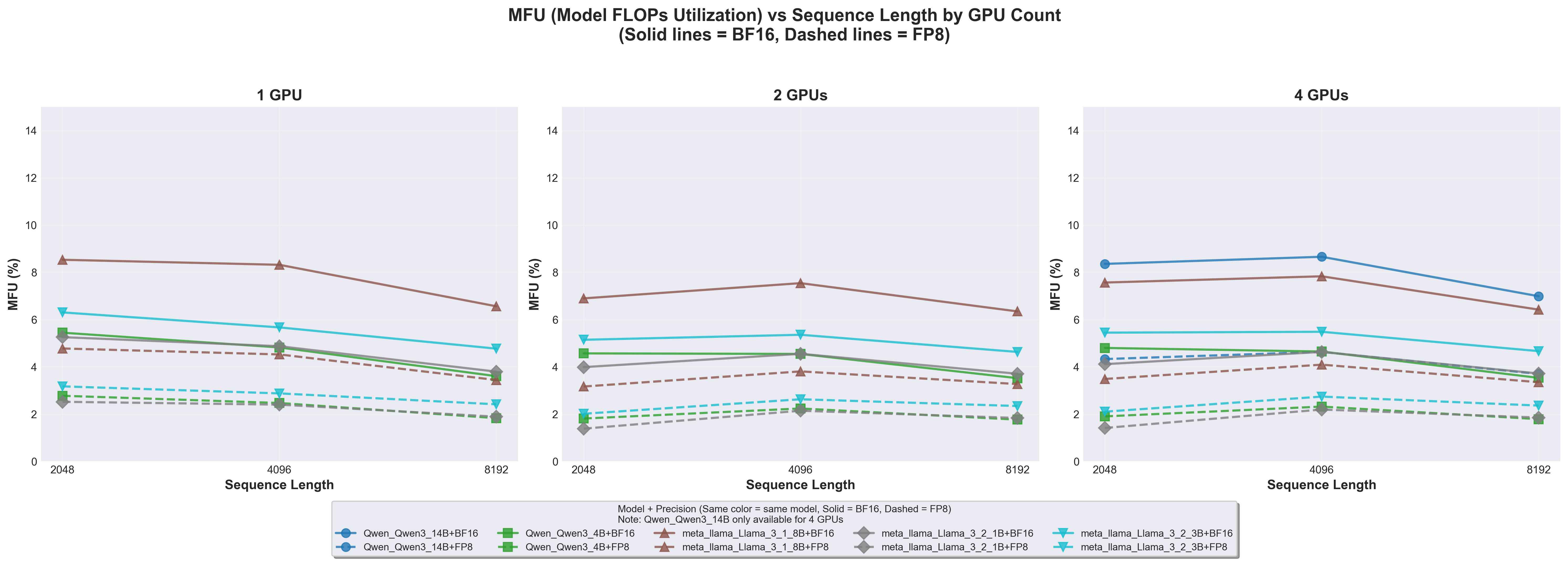
9.4 Hardware Utilization: MFU Analysis
MFU vs Sequence Length
9.4.1 Key Findings
Overall MFU is very low: 2-9%
Expected given batch_size=1 constraint
B200’s 9000 TFLOPs peak severely underutilized
Llama 3.1 8B achieves highest MFU: ~8-9%
Larger models better utilize tensor cores
Higher arithmetic intensity
MFU peaks at sequence length 4096
Matches TFLOPs sweet spot
Best balance of compute vs memory
FP8 and BF16 show nearly identical MFU
Both ~4-8% depending on model
FP8’s higher peak TFLOPs offset by higher achieved TFLOPs
Modern GPUs are designed for massive parallelism: - B200 can process 100,000+ tokens in parallel - batch_size=1 × seq_len=8192 = only 8,192 tokens - ~99% of GPU capacity idle!
Additional factors:
Non-compute operations: Data loading, normalization (no FLOPs)
Our 2-9% MFU is expected and acceptable for this benchmark’s goals.
9.5 Training Quality: The Critical Finding
This section presents our most significant empirical finding: the dramatic difference in FP8 vs BF16 training quality between single-GPU and multi-GPU configurations.
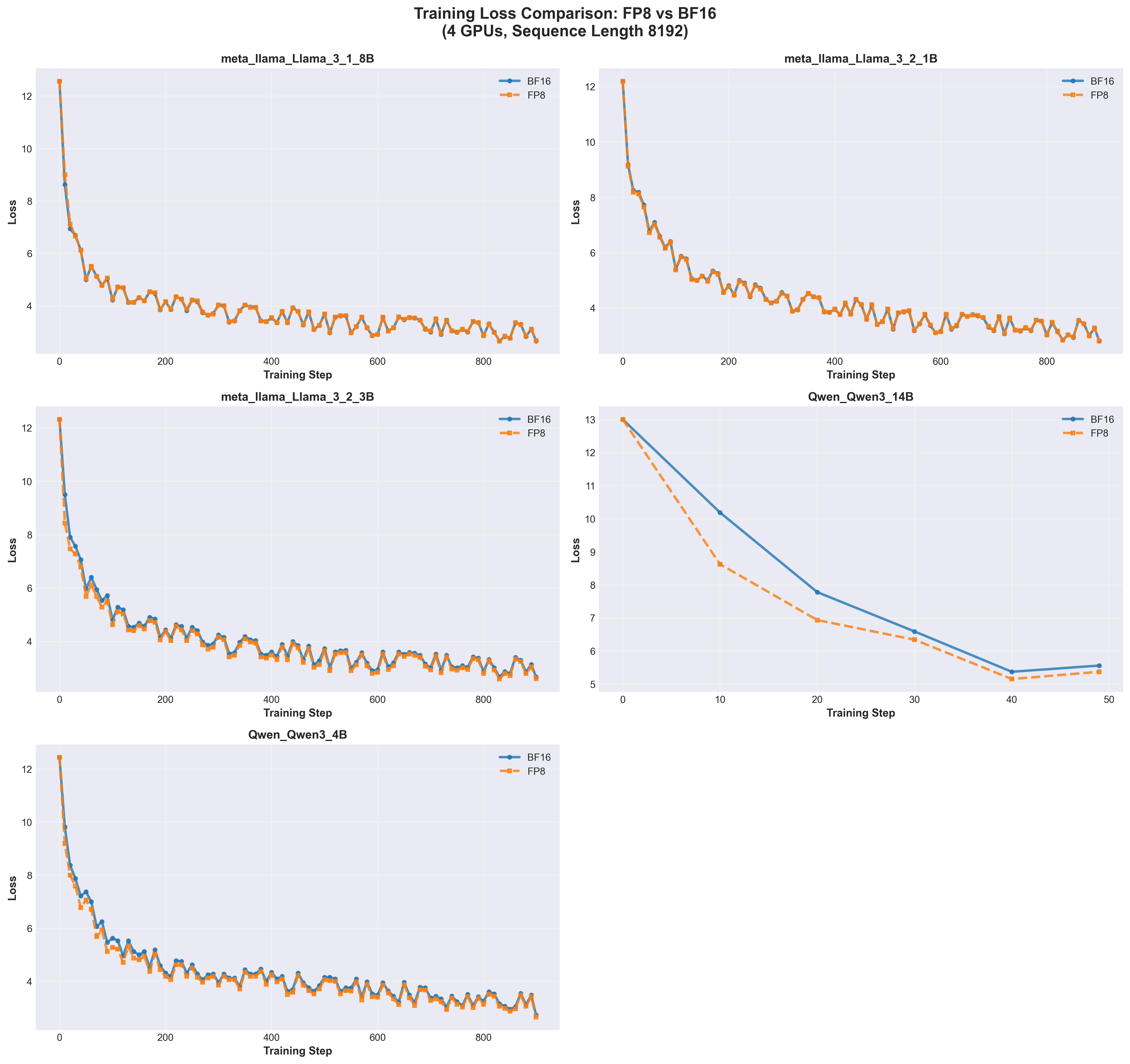
9.5.1 Four GPUs: FP8 and BF16 Equivalent
Loss Comparison 4 GPUs
Key Observations:
FP8 and BF16 curves are virtually identical
All models converge from loss ~12-13 to ~3-6
No evidence of FP8 training instability
Curves overlap throughout training
Model-specific convergence rates:
Llama 3.1 8B: Fastest convergence (loss ~3 by step 200)
Llama 3.2 1B/3B: Moderate convergence (loss ~3-4 by step 200)
Qwen3 14B: Slower initial drop but smoothest curve
Qwen3 4B: Similar to Llama 3.2 3B
Smooth loss curves across all models
Minimal oscillation
Consistent downward trend
No precision-related instabilities
Implication:FP8 is production-ready for multi-GPU training with no quality degradation.
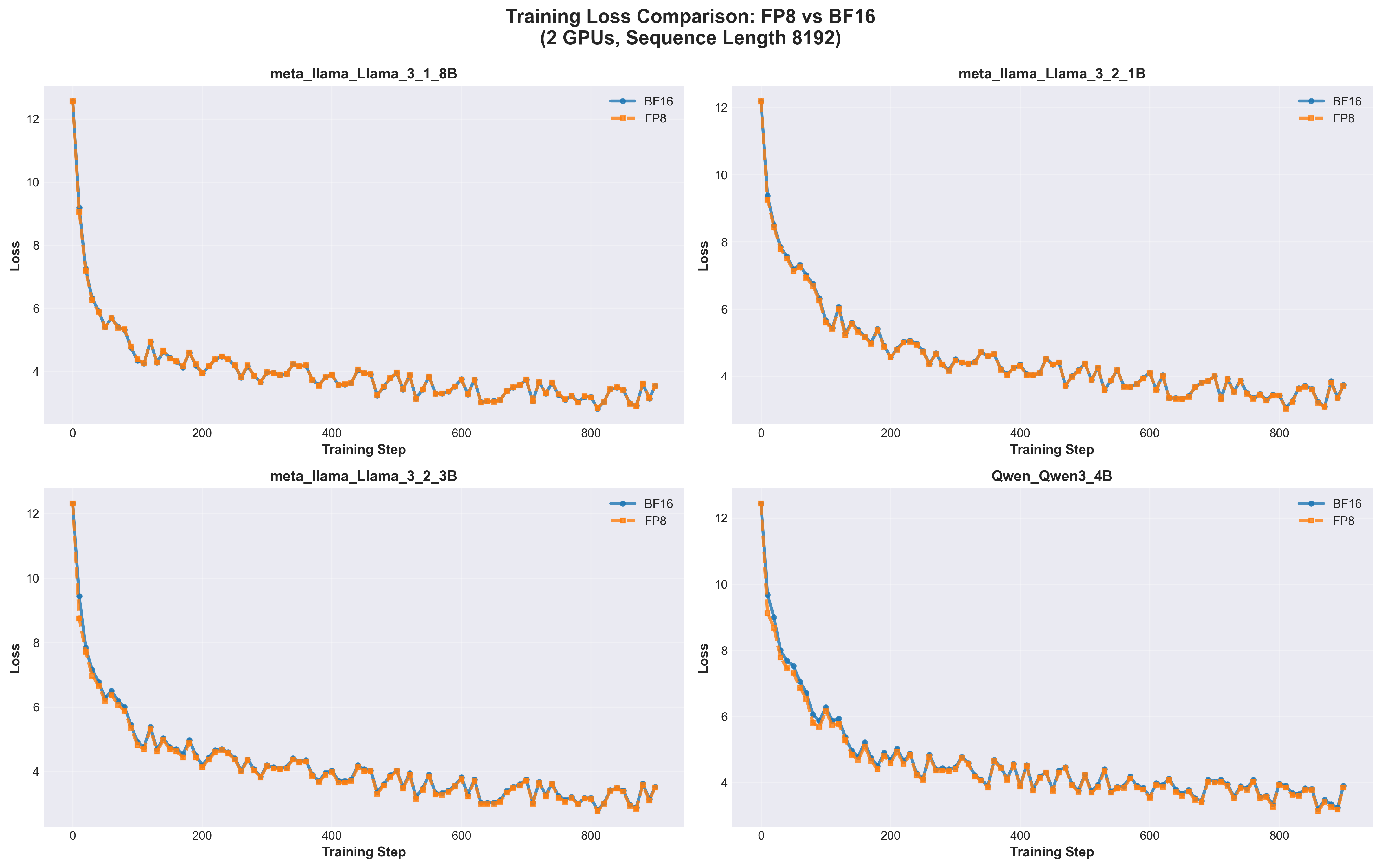
9.5.2 Two GPUs: FP8 Remains Comparable
Loss Comparison 2 GPUs
Key Observations:
FP8 and BF16 still highly comparable
Nearly overlapping loss curves
All models converge successfully
Slightly more oscillation than 4-GPU case
Visible in later training steps (after step 400)
Affects both precisions equally
Not a precision issue but gradient noise
Convergence patterns match 4-GPU results
Final loss values similar
No systematic FP8 disadvantage
Implication:2 GPUs is sufficient for FP8 training with batch_size=1 per GPU.
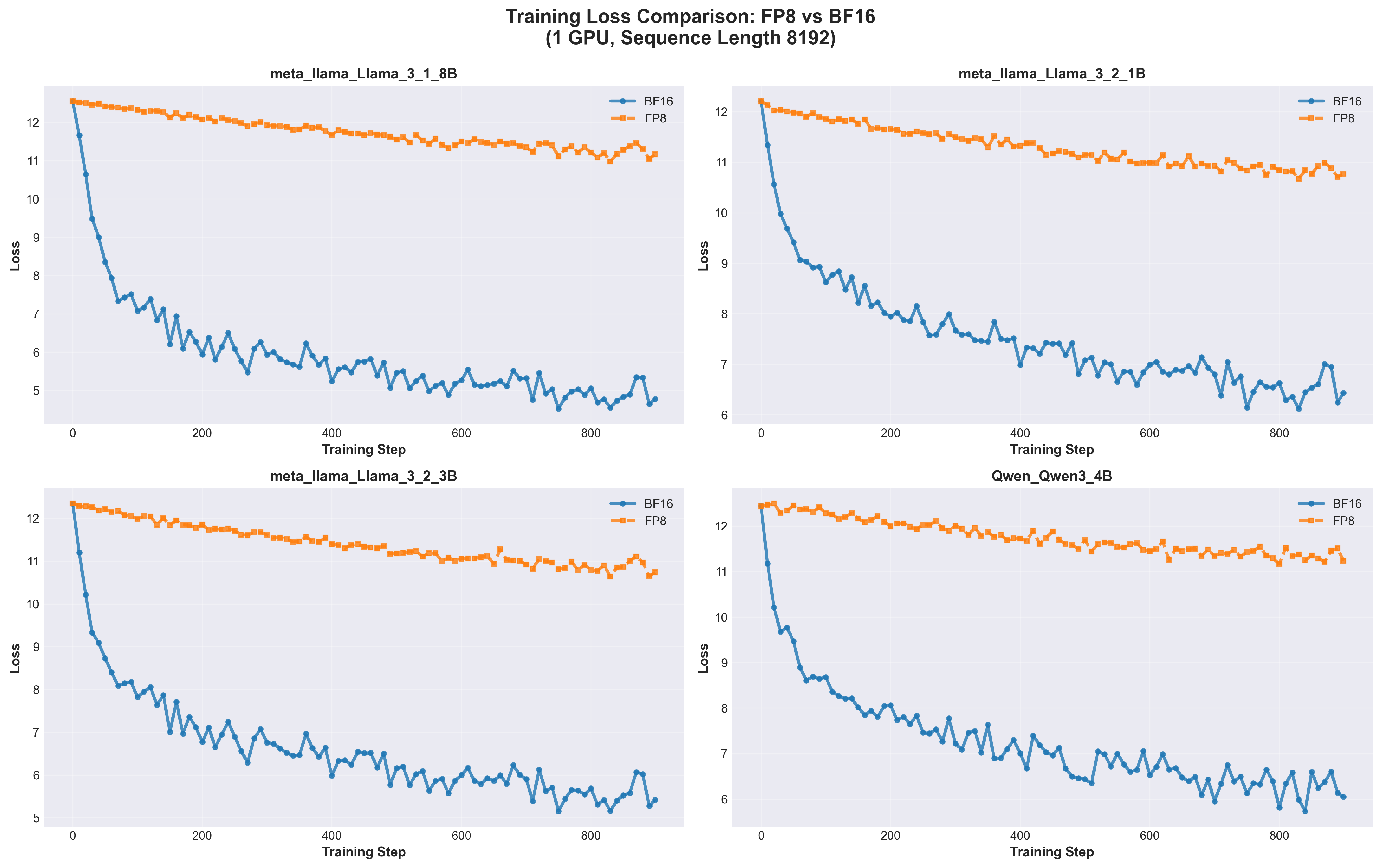
9.5.3 Single GPU: BF16 Dramatically Outperforms FP8
Loss Comparison 1 GPU
Key Observations:
BF16 significantly outperforms FP8 on all models
BF16 converges to loss ~5-7
FP8 plateaus at loss ~11-12
Gap: 4.5-6.5 loss units
FP8 shows minimal learning progress
Initial drop from 12.5 → 11.5
Then plateaus with no further improvement
Fails to learn effectively
BF16 demonstrates smooth convergence
Consistent downward trend
Reaches good loss values
Normal training dynamics
Gap is consistent across all models
Not model-specific
Fundamental interaction between precision and batch size
Model-Specific Results:
Model
BF16 Final Loss
FP8 Final Loss
Gap
Llama 3.1 8B
~5.0
~11.5
~6.5
Llama 3.2 1B
~6.5
~11.0
~4.5
Llama 3.2 3B
~5.5
~11.0
~5.5
Qwen3 4B
~6.5
~11.5
~5.0
Implication:Never use FP8 for single-GPU training with small batches.
9.6 The Precision-Noise Trade-off: Theoretical Analysis
9.6.1 Why Does FP8 Fail on 1 GPU but Succeed on 2+ GPUs?
This is the most important theoretical insight from our benchmark. The answer lies in the interaction between numerical precision and gradient estimation quality.
9.6.2 Gradient Noise Dominates at Batch Size 1
Stochastic Gradient Descent (SGD) relies on gradient estimates:
True gradient = E[∇L(θ, x)]  (expectation over all data)
Estimated gradient = ∇L(θ, x_batch)  (gradient from batch)
With batch_size=1:
Each gradient comes from a single sample
Extremely high variance (single sample cannot represent distribution)
# Single sample gradient (batch_size=1)grad_sample_1 = [0.5, -2.3, 0.1, ...] # High variancegrad_sample_2 = [-0.3, 1.8, -0.5, ...] # Very different!grad_sample_3 = [0.8, -0.5, 0.3, ...] # Also very different!# True gradient (average of many samples)grad_true = [0.3, -0.4, 0.1, ...] # Much more stable
9.6.3 2. FP8’s Limited Precision Amplifies the Noise
FP8 quantization introduces errors:
Precision comparison:
FP32: 23-bit mantissa (~7 decimal digits)
BF16: 7-bit mantissa (~3 decimal digits)
FP8: 2-3 bit mantissa (~1-2 decimal digits)
FP8 quantization errors:
# BF16 → FP8 conversion loses precisiontrue_gradient =0.000123456 (BF16)fp8_gradient =0.000123 (FP8, rounded)error =0.000000456 (quantization error)# Small values critical for optimization are lost!small_component =0.00001 (BF16)fp8_component =0.0 (FP8, underflow!)
When noise is high (batch_size=1):
FP8’s precision is insufficient to preserve gradient signal
Important small gradient components lost to quantization
Optimization cannot make progress
9.6.4 Multi-GPU Gradient Averaging as Noise Reduction
9.6.5 Mathematical Framework: The Precision-Noise Trade-off
We can formalize this as:
Total Optimization Error = Gradient Sampling Noise + Numerical Precision Error

Single GPU (batch_size=1):
  Sampling Noise: HIGH (σ²)
  Precision Error: MEDIUM (FP8 quantization)
  Total Error: HIGH + MEDIUM = TOO HIGH for learning ❌

2 GPUs (batch_size=1 each):
  Sampling Noise: MEDIUM (σ²/2)
  Precision Error: MEDIUM (FP8 quantization)
  Total Error: MEDIUM + MEDIUM = ACCEPTABLE ✅

4 GPUs (batch_size=1 each):
  Sampling Noise: LOW (σ²/4)
  Precision Error: MEDIUM (FP8 quantization)
  Total Error: LOW + MEDIUM = GOOD ✅
Phase transition: At some point (between 1 and 2 GPUs), total error drops below the threshold needed for effective learning.
9.6.6 Why BF16 is More Robust on Single GPU
BF16 advantages:
8-bit exponent (same range as FP32)
7-bit mantissa (4-8x more precision than FP8’s 2-3 bits)
Can represent wide dynamic range simultaneously
Numerical example:
Gradient component:     0.000123456
BF16 representation:    0.000123
FP8 representation:     0.000120  (or 0.0000 if underflow)

BF16 error: 0.456e-6    (tiny)
FP8 error:  3.456e-6    (significant) or total loss
BF16’s extra precision:
Preserves small but important gradient components
Handles outlier values better
Less sensitive to scaling issues
Sufficient precision even with high noise
9.6.7 Empirical Validation
Our results empirically validate this theory:
Configuration
Effective Batch
Gradient Variance
FP8 Performance
1 GPU
1
Very High (σ²)
❌ Fails (loss ~11)
2 GPUs
2
Medium (σ²/2)
✅ Works (loss ~3)
4 GPUs
4
Low (σ²/4)
✅ Works (loss ~3)
Phase transition observed:
1 GPU: Total error too high for FP8
2 GPUs: Total error acceptable for FP8
The transition happens between 1 and 2 GPUs
9.6.8 Practical Recommendations
For FP8 Training:
✅ Use FP8 when:
Multi-GPU training (2+ GPUs with FSDP/DDP)
Batch size ≥ 4 per GPU
Gradient accumulation over multiple micro-batches
Training at scale (communication bandwidth matters)
❌ Avoid FP8 when:
Single GPU with batch_size ≤ 2
Tasks requiring maximum numerical precision
Early research with minimal infrastructure
Minimum recommended configurations:
# Option 1: Multi-GPU (minimum 2 GPUs)batch_size_per_gpu =1# Acceptable with 2+ GPUsnum_gpus =2# Minimum for FP8effective_batch_size =2# Option 2: Single GPU with larger batchbatch_size_per_gpu =4# Minimum for single GPU FP8num_gpus =1effective_batch_size =4# Option 3: Gradient accumulationbatch_size_per_gpu =1accumulation_steps =4# Simulate effective_batch_size=4num_gpus =1
For Production Training:
Typical settings:
8-64 GPUs
batch_size = 1-4 per GPU
Effective batch size = 8-256
FP8 works excellently in this regime
9.7 Summary of Experimental Findings
9.7.1 Performance Metrics Summary
Metric
FP8 vs BF16
Optimal Sequence Length
Multi-GPU Scaling
TFLOPs
FP8 +10-15%
4096
Good (3.5-3.8x on 4 GPUs)
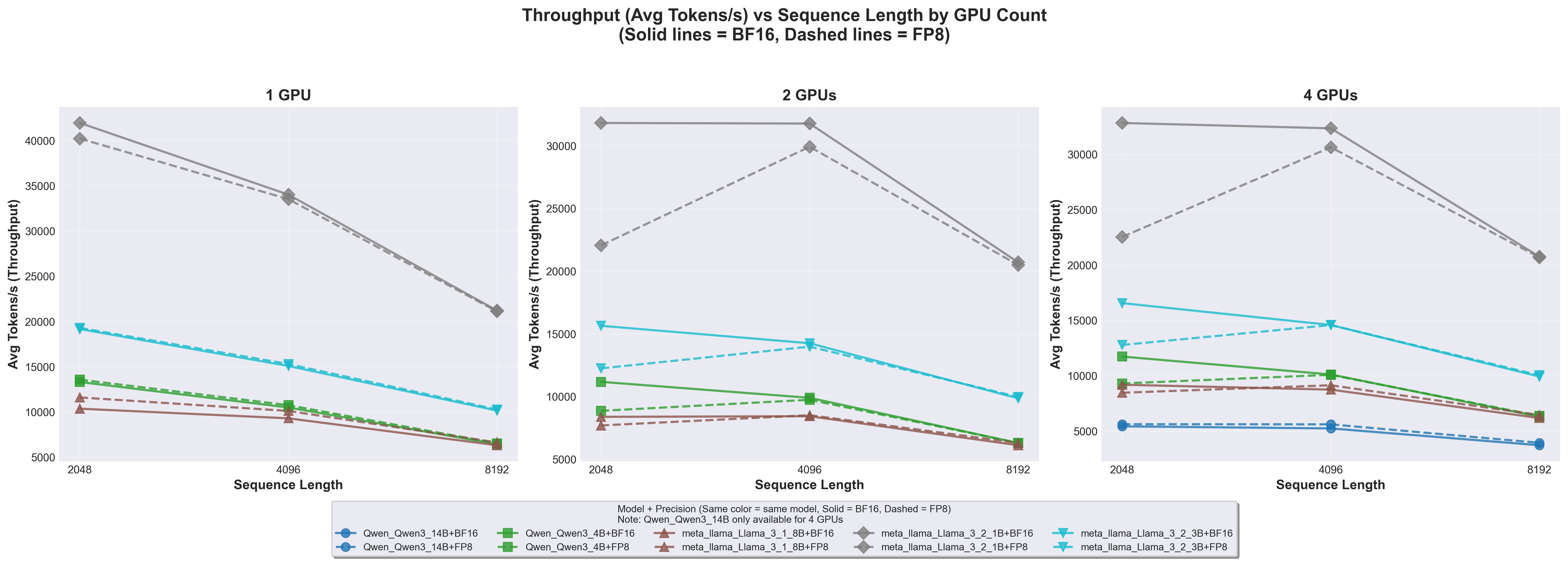
Tokens/s
Comparable
2048 (highest)
Sublinear (batch_size=1)
MFU
Comparable (2-9%)
4096
Marginal improvement
9.7.2 Training Quality Summary
GPU Count
FP8 vs BF16
Gradient Variance
Recommendation
1 GPU
BF16 ≫ FP8
Very High
Never use FP8
2 GPUs
FP8 ≈ BF16
Medium
Minimum for FP8
4 GPUs
FP8 = BF16
Low
Ideal for FP8
9.7.3 Key Insights
FP8 is production-ready for multi-GPU training (2+ GPUs)
Batch size is critical for FP8 stability, not just throughput
Sequence length 4096 offers best TFLOPs/MFU balance
Low MFU (2-9%) is expected with batch_size=1
Gradient averaging compensates for FP8 precision in distributed training
10 Conclusions
Our comprehensive benchmark of FP8 training on NVIDIA B200 GPUs reveals several critical insights that advance both the practical deployment and theoretical understanding of low-precision training for large language models. FP8 delivers measurable performance gains across all tested configurations, achieving 10-15% higher computational throughput (TFLOPs) compared to BF16, along with a 2x reduction in communication bandwidth when using enable_fsdp_float8_all_gather=True and 50% memory savings for parameters and activations. However, our most important finding centers on the interaction between numerical precision and gradient estimation quality: FP8 training quality is not solely determined by bit precision, but rather by the interplay between precision limitations and gradient noise. On multi-GPU configurations (2 or more GPUs), FP8 achieves training quality equivalent to BF16, with loss curves that track nearly perfectly throughout training, while single-GPU training with small batch sizes shows BF16 significantly outperforming FP8, with FP8 models plateauing at loss values 4-6 units higher. This phenomenon stems from gradient averaging in distributed training acting as essential noise reduction that compensates for FP8’s precision limitations, explaining why FP8 has become practical primarily in the era of large-scale distributed training. For practitioners, these results translate to clear deployment guidelines: FP8 should be used for multi-GPU training with FSDP2 or DDP (minimum 2 GPUs), production-scale training (8+ GPUs), memory-constrained scenarios, and communication-bound workloads, while BF16 remains preferable for single-GPU training with small batches, early research and prototyping, and tasks requiring maximum precision. Key configuration recommendations include maintaining a minimum effective batch size of 4, using sequence lengths of 2048-4096 tokens for optimal efficiency, skipping first and last layer FP8 conversion for stability, and enabling enable_fsdp_float8_all_gather=True for communication bandwidth savings.
The role of hardware interconnect emerged as a crucial consideration. Our excellent multi-GPU scaling results (88-95% efficiency on 4 GPUs) were achieved with NVLink connectivity providing 900 GB/s bandwidth per GPU. Systems using standard PCIe interconnect (128 GB/s per GPU) should expect 20-40% lower multi-GPU throughput and degraded scaling efficiency of 50-70%. On such systems, FP8’s communication bandwidth advantages become even more critical, potentially shifting the cost-benefit analysis in favor of low-precision training despite compute-bound workloads.
Several limitations of this study must be acknowledged. Our intentional use of batch size 1, while valuable for isolating sequence length effects and revealing precision sensitivity, does not represent production training practices where batch sizes of 4-8 per GPU are standard. The short training runs (50-1000 steps) and use of random initialization, though sufficient for performance benchmarking and convergence trend analysis, cannot speak to final model quality or long-term training stability over billions of steps. The TinyStories dataset, while convenient for benchmarking, may not expose all numerical stability issues present in diverse production datasets. Finally, our focus on models up to 14B parameters leaves open questions about how FP8 behaves at the 70B-405B parameter scales common in production systems.
The dramatic difference between single-GPU and multi-GPU FP8 performance reveals a deep connection between numerical precision and gradient estimation quality in stochastic optimization. This finding has implications beyond FP8, informing our understanding of how low-precision arithmetic interacts with the fundamental dynamics of deep learning. The precision-noise trade-off we documented provides empirical evidence for theoretical frameworks in stochastic optimization, demonstrating that required numerical precision scales with gradient noise levels. As large language models continue to grow and training costs escalate into millions of dollars, techniques like FP8 training will become increasingly important for making cutting-edge AI research accessible to a broader community.
11 Future Research Directions
The findings from this benchmark open several promising avenues for future investigation, each addressing limitations of the current work while building on the insights gained about FP8 training dynamics. The question of optimal batch size for single-GPU FP8 training remains open, with our results showing a clear phase transition between ineffective training at batch size 1 and effective training at larger batch sizes, warranting systematic exploration to identify the precise threshold where FP8 becomes viable in resource-constrained environments. FP8 for fine-tuning represents largely unexplored territory, as pretrained weights exhibit specific learned distributions that may interact differently with FP8 quantization compared to random initialization, with critical questions including whether FP8 preserves pretrained knowledge, how it interacts with parameter-efficient methods like LoRA and QLoRA, and whether certain layers show heightened sensitivity during fine-tuning. Scaling to very large models of 70B-405B parameters represents the next frontier, where testing across multi-node training setups would reveal how FP8 interacts with other essential optimizations like Flash Attention and gradient checkpointing, with the hypothesis that FP8 advantages may become more pronounced at larger scales where communication bandwidth and memory capacity become primary bottlenecks. The choice of optimizer may significantly impact FP8 training dynamics, as alternatives to AdamW such as Lion, Adafactor, and Sophia exhibit different numerical characteristics that could interact differently with reduced precision, raising questions about whether simpler optimizers work better with FP8 and whether optimizer states themselves can be quantized. Mixed precision strategies offering finer granularity than all-or-nothing FP8 deserve investigation, with approaches like selectively maintaining critical layers in BF16 while using FP8 for large feedforward networks, or dynamically adjusting precision during training, potentially delivering better quality than full FP8 while achieving more memory savings than full BF16. Hardware comparisons across AMD’s MI300X, Google’s TPU v5, and Intel’s Gaudi2 would provide valuable context for generalizability, revealing whether our findings are NVIDIA-specific or represent universal properties of FP8 training while informing hardware selection decisions. Production deployment case studies spanning weeks or months on production datasets would validate whether FP8’s advantages persist over billions of training steps, with comprehensive cost-benefit analysis measuring training time, monetary cost, energy consumption, and downstream task performance providing the economic data necessary for informed precision choices. The convergence of these investigations would provide comprehensive understanding of FP8 training across the full spectrum of practical applications, from resource-constrained single-GPU research to massive-scale production training, proving essential as the field continues pushing toward larger models and more efficient training methods while managing computational costs and environmental impact.
# Single model, single configurationaccelerate launch --num_processes=4 fp8_benchmark.py \ meta-llama/Llama-3.2-1B \--sequence-length 8192 \--precision fp8 \--num-steps 1000# Run full sweepbash run_sweep.sh
13.3 Hardware Requirements
Minimum: 1x NVIDIA H100 or B200 (80GB+)
Recommended: 4x NVIDIA B200 (180GB) for full benchmark
Storage: 50GB for models and datasets
RAM: 128GB+ system RAM
14 Acknowledgments
We thank:
HuggingFace for the excellent Accelerate library and examples
PyTorch team for torchao and FSDP2 implementation
NVIDIA for B200 GPU architecture and FP8 support
Lambda Labs for providing GPU cloud infrastructure
Open-source community for models, datasets, and tools
This blog post is based on research conducted in December 26-28, 2025 using NVIDIA B200 GPUs. Results may vary on different hardware configurations and your moods
Source Code
---title: "Pre-Training Large Language Models with FP8: A Comprehensive Benchmark on NVIDIA B200 GPUs"description: "A comprehensive guide to FP8 (8-bit floating point) training for large language models, exploring performance benefits and implementation strategies on NVIDIA B200 GPUs"author: "Dipankar Baisya"date: "2025-12-30"categories: [deep-learning, fp8, low-precision, pytorch, optimization]format: html: code-fold: false code-tools: true toc: true toc-depth: 2 number-sections: true---{{< include ./fp8_blog.md >}}