1 Introduction

This study presents a comprehensive analysis of distributed training strategies for large language models using PyTorch. Three distributed training approaches—Data Parallel (DDP), Fully Sharded Data Parallel with full parameter sharding (FSDP-Full/ZeRO-3), and FSDP with gradient sharding only (FSDP-Grad/ZeRO-2)—were implemented and evaluated against a single-GPU baseline. Experiments conducted on a 2x H100 SXM5 Lambda instance training GPT-2 Large (774M parameters) reveal that FSDP-Grad achieves 97.71% compute efficiency, nearly matching single-GPU performance while providing memory savings and enabling larger-scale training.

Training large language models has become increasingly challenging as model sizes grow from millions to billions of parameters. A GPT-2 Large model with 774M parameters requires approximately 12GB of GPU memory for training on a single GPU. This memory consumption breaks down as follows: model parameters stored in FP32 format consume ~3GB (774M × 4 bytes), gradients of the same size add another ~3GB, optimizer states (momentum and variance for AdamW) require ~6GB (2× parameters in FP32), totaling ~12GB for the model states alone. Additionally, activation tensors saved during the forward pass for backpropagation require extra memory that scales with batch size and sequence length. As models scale to billions or trillions of parameters, this linear memory growth makes single-GPU training infeasible, necessitating distributed training strategies.

This comprehensive study aims to: (1) Implement and compare three distributed training strategies: DDP, FSDP-Full (ZeRO-3), and FSDP-Grad (ZeRO-2); (2) Analyze memory consumption, throughput, and communication patterns for each approach; (3) Profile GPU utilization, compute vs. communication time, and operator-level performance; and (4) Provide practical recommendations for choosing the optimal strategy based on model size and hardware constraints.

The experimental setup utilized a GPU 2x H100 SXM5 Lambda instance with 2x NVIDIA H100 GPUs (80GB HBM3 each) connected via NVLink/NVSwitch for high-bandwidth GPU-to-GPU communication. The model configuration consisted of GPT-2 Large architecture with 774,439,808 parameters, sequence length of 1024 tokens, global batch size of 32, micro batch size of 8 per GPU, 20 training steps, and learning rate of 3e-4 with cosine annealing. The software stack included PyTorch 2.x with CUDA support, uv for Python package management, NCCL (NVIDIA Collective Communications Library) as the distributed backend, and PyTorch Profiler with Chrome trace export for profiling.

2 Challenges in Distributed Training vs. Single GPU Training

2.1 Memory Constraints

2.1.1 Single GPU Training

Training a neural network on a single GPU requires storing:

Model Parameters (W): Original weights
Gradients (∇W): Same size as parameters
Optimizer States (O): For Adam/AdamW, stores first and second moments (2x parameter size)
Activations (A): Intermediate outputs saved for backward pass

For GPT-2 Small (124,439,808 parameters, or ~124M) with mixed precision training:

Parameters:       474.70 MB  (124M × 4 bytes in FP32)
Gradients:        474.70 MB  (same size as parameters)
Optimizer States: 949.40 MB  (FP32: momentum + variance = 2× parameters)
Total Estimated:  1,898.80 MB
Actual Peak:      3,076.27 MB (includes activations and overhead)

The parameter memory calculation: 124,439,808 parameters × 4 bytes (FP32) = 497,759,232 bytes ≈ 474.70 MB. Despite using mixed precision (FP16 for forward/backward passes), the optimizer maintains an FP32 master copy of weights, so the base parameter storage is FP32.

The 1,177.47 MB difference between estimated and actual memory comes from:

Activation tensors stored during forward pass (~800-900 MB)
Temporary buffers for operations
PyTorch framework overhead
Memory fragmentation

2.1.2 Distributed Training Challenges

When scaling to multiple GPUs, new challenges emerge:

1. Data Parallelism Memory Replication Traditional DDP replicates the entire model on each GPU, which doesn’t reduce per-GPU memory usage—it only enables larger batch sizes.

2. Communication Overhead Distributed training introduces collective communication operations: - All-Reduce: Synchronize gradients across all GPUs (DDP) - All-Gather: Collect sharded parameters/gradients from all GPUs (FSDP) - Reduce-Scatter: Reduce and distribute results across GPUs (FSDP)

3. Synchronization Barriers GPUs must wait for each other at communication points, potentially causing idle time if workloads are imbalanced.

4. Network Bandwidth The data transfer rate between GPUs, measured in GB/s (gigabytes per second). Higher bandwidth enables faster gradient/parameter synchronization. H100s use NVLink (900 GB/s bidirectional), allowing near-simultaneous compute and communication. Lower bandwidth (e.g., PCIe: 32 GB/s) creates bottlenecks where GPUs wait idle during all-reduce/all-gather operations.

5. Load Balancing Uneven data distribution or computational load can cause some GPUs to finish early and wait idle.

2.2 Communication vs. Computation Trade-off

The fundamental challenge in distributed training is hiding communication latency behind computation. Ideal distributed training achieves:

Compute Efficiency = (Compute Time) / (Total Time) × 100%

Where Total Time = Compute Time + Communication Time + Idle Time.

Single GPU Baseline: - Compute: 97.87% - Communication: 1.16% (memory transfers, kernel overhead) - Idle: 0.97%

Distributed Training Goal: Match or approach baseline efficiency while enabling: - Training models that don’t fit on a single GPU - Faster training through data parallelism - Flexibility to scale to larger clusters

2.3 Gradient Accumulation and Synchronization

2.3.1 Single GPU Approach

Gradient accumulation simply accumulates gradients over multiple micro-batches before updating weights:

for micro_batch in range(grad_accumulation_steps):
    loss = forward_backward(micro_batch)
    loss.backward()  # Accumulate gradients
optimizer.step()  # Update weights
optimizer.zero_grad()

2.3.2 Distributed Training Synchronization

Must decide when to synchronize gradients:

The Synchronization Problem

Synchronizing every micro-batch wastes bandwidth
Using no_sync() context manager prevents unnecessary all-reduce operations
Only synchronize on the last micro-batch of gradient accumulation

Here’s the optimized approach:

for i, micro_batch in enumerate(batches):
    is_last = (i + 1) % grad_accumulation_steps == 0

    if not is_last:
        with model.no_sync():  # Skip gradient synchronization
            loss.backward()
    else:
        loss.backward()  # Synchronize gradients across GPUs

This optimization reduces communication overhead significantly. The experimental results show that DDP with proper gradient accumulation achieves 97.36% compute efficiency.

2.4 Memory Sharding Strategies

To overcome memory limitations, Fully Sharded Data Parallel (FSDP) implements the ZeRO (Zero Redundancy Optimizer) approach:

Component	DDP (No Sharding)	FSDP-Grad (ZeRO-2)	FSDP-Full (ZeRO-3)
Parameters	Replicated	Replicated	Sharded
Gradients	Synchronized	Sharded	Sharded
Optimizer States	Replicated	Sharded	Sharded
Memory per GPU	100%	~67%	~33%
Communication	All-Reduce	All-Gather (grads)	All-Gather (params) + Reduce-Scatter (grads)

Table 1: Comparison of Memory Sharding Strategies for Distributed Training

For GPT-2 Large on 2 GPUs: - DDP: 12GB per GPU (no savings) - FSDP-Grad: ~8GB per GPU (1.5x reduction) - FSDP-Full: ~4GB per GPU (3x reduction)

The Trade-off

More aggressive sharding reduces memory but increases communication frequency and complexity.

3 Distributed Training Approaches

3.1 Baseline: Single GPU Training

The baseline implementation serves as the reference point for performance comparison.

Implementation (train_baseline.py):

# Device setup
device = "cuda" if torch.cuda.is_available() else "cpu"

# Model initialization
config = AutoConfig.from_pretrained("gpt2-large")
model = MyGPT2LMHeadModel(config)
model.init_weights()
model = model.to(device)

# Gradient accumulation to match distributed global batch size
global_batch_size = 32
micro_batch_size = 8
grad_acc_steps = global_batch_size // micro_batch_size  # 4 steps

# Training loop with gradient accumulation
for batch in dataloader:
    loss = model(batch)
    scaled_loss = loss / grad_acc_steps
    scaled_loss.backward()

    if (step + 1) % grad_acc_steps == 0:
        optimizer.step()
        optimizer.zero_grad()

Key Characteristics:

Simple, straightforward implementation
No communication overhead
Limited by single GPU memory capacity
Serves as performance upper bound (97.87% compute efficiency)

Performance Metrics:

Training Time: 112.3s for 20 steps
Peak Memory: 3,076 MB
Compute Efficiency: 97.87%
Throughput: 32,582 tokens/sec (batch size 8)

3.2 Data Parallel (DDP)

3.2.1 Concept

DDP replicates the model on each GPU and synchronizes gradients after the backward pass using an all-reduce collective operation.

How It Works:

Each GPU maintains a complete copy of the model
Each GPU processes a different subset of the data (data parallelism)
After backward pass, gradients are averaged across all GPUs using all-reduce
All GPUs update their models identically using synchronized gradients

3.2.2 Implementation

import torch.distributed as dist
from torch.nn.parallel import DistributedDataParallel as DDP

# Initialize distributed process group
dist.init_process_group(backend='nccl')
rank = dist.get_rank()
world_size = dist.get_world_size()
local_rank = int(os.environ['LOCAL_RANK'])

# Set device for this process
torch.cuda.set_device(local_rank)
device = f'cuda:{local_rank}'

# Critical: All ranks must use same seed for identical initialization
torch.manual_seed(42)
torch.cuda.manual_seed(42)

# Create model and wrap with DDP
model = MyGPT2LMHeadModel(config)
model.init_weights()
model = model.to(device)
model = DDP(model, device_ids=[local_rank])

3.2.3 Key Implementation Detail: Gradient Synchronization with `no_sync()`

From distributed_trainer.py:

def training_step(self, inputs, targets, should_sync: bool):
    """
    Training step with DDP no_sync support.

    Key concept: For gradient accumulation, we only sync gradients
    on the last micro-batch to avoid unnecessary communication overhead.
    """
    # Forward pass
    logits = self.model(inputs)
    loss = nn.functional.cross_entropy(
        logits.view(-1, logits.size(-1)),
        targets.view(-1)
    )

    # Backward with conditional synchronization
    scaled_loss = loss / self.grad_accumulation_steps

    if self.ddp_enabled and not should_sync:
        # Don't sync gradients for intermediate micro-batches
        with self.model.no_sync():
            scaled_loss.backward()
    else:
        # Sync gradients on last micro-batch (triggers all-reduce)
        scaled_loss.backward()

    return loss

Why no_sync() Matters

Without this optimization, DDP would perform all-reduce after every backward() call:

With 4 micro-batches per step: 4 × all-reduce operations
With no_sync(): Only 1 all-reduce operation (on the last micro-batch)
Result: 4x reduction in communication overhead

3.2.4 Communication Pattern

Operation: All-Reduce (averages gradients across all ranks)
Frequency: Once per gradient accumulation cycle (every 2 micro-batches with 2 GPUs)
Data Volume: All gradient tensors (~475 MB)
NCCL Implementation: Ring all-reduce algorithm

3.2.5 Performance Metrics

Training Time: 58.3s (1.93x speedup over baseline)
Communication Overhead: 105.3 ms
Compute Efficiency: 97.36%
Communication Overlap: 92.50%

3.2.6 Advantages & Limitations

Advantages:

✅ Simple to implement (single DDP() wrapper)

✅ Excellent performance when model fits in memory

✅ Minimal code changes from single-GPU training

Limitations:

❌ No memory savings (full model replication)

❌ Highest communication overhead among strategies tested

❌ Doesn’t scale to models larger than single GPU capacity

3.3 Fully Sharded Data Parallel - Full Sharding (FSDP-Full / ZeRO-3)

3.3.1 Concept

FSDP-Full implements ZeRO Stage 3, sharding parameters, gradients, and optimizer states across all GPUs. Each GPU only stores a fraction of the model, reconstructing full parameters on-demand during forward/backward passes.

How It Works:

Model parameters are sharded across GPUs (each GPU holds 1/N of weights)
Before each layer’s forward pass: all-gather to reconstruct full parameters
After forward pass: parameters are freed, only shards retained
Before backward pass: all-gather parameters again
After backward pass: reduce-scatter to shard gradients across GPUs
Optimizer updates only local parameter shards

3.3.2 Implementation

from torch.distributed.fsdp import FullyShardedDataParallel as FSDP
from torch.distributed.fsdp import ShardingStrategy

def setup_fsdp_model(model, device, sharding_strategy_name='FULL_SHARD'):
    """
    Wrap model with FSDP using per-layer wrapping.

    Sharding strategies:
    - FULL_SHARD: Parameters, gradients, optimizer states all sharded
      -> Max memory savings, more communication
    - SHARD_GRAD_OP: Only gradients and optimizer states sharded
      -> Moderate savings, less communication
    """
    model = model.to(device)

    strategy_map = {
        'FULL_SHARD': ShardingStrategy.FULL_SHARD,
        'SHARD_GRAD_OP': ShardingStrategy.SHARD_GRAD_OP,
        'NO_SHARD': ShardingStrategy.NO_SHARD
    }
    sharding_strategy = strategy_map[sharding_strategy_name]

    # Per-layer wrapping for fine-grained control
    # Each transformer block is wrapped individually
    for i, block in enumerate(model.transformer.h):
        model.transformer.h[i] = FSDP(
            block,
            sharding_strategy=sharding_strategy
        )

    # Wrap entire model
    model = FSDP(model, sharding_strategy=sharding_strategy)

    return model

Per-Layer Wrapping is Critical

Per-layer wrapping enables:

Granular Memory Management: Each transformer block can independently gather/shard parameters
Better Overlap: While layer N is computing, layer N+1 can prefetch parameters
Reduced Peak Memory: Only one layer’s full parameters need to be materialized at a time
Communication Efficiency: Smaller, more frequent all-gathers overlap better with computation

3.3.3 Communication Pattern

For a 36-layer GPT-2 Large model:

All-Gather Operations: ~73 calls (forward + backward for each layer)
- Each call gathers 1/N parameters from all GPUs
- Total duration: 50,074 μs (50.1 ms)
- Average per call: ~686 μs
Reduce-Scatter Operations: Shard and reduce gradients

3.3.4 Memory Breakdown (per GPU, 2 GPUs total)

Parameters:  6 GB / 2 = 3 GB per GPU (sharded)
Gradients:   6 GB / 2 = 3 GB per GPU (sharded)
Optimizer:   2 GB / 2 = 1 GB per GPU (sharded)
Activations: ~1.5 GB per GPU (not sharded)
Peak Memory: ~4 GB per GPU (3x reduction vs. baseline)

3.3.5 Performance Metrics

Training Time: 58.8s (1.91x speedup)
Communication Overhead: 94.7 ms
Compute Efficiency: 96.98%
Communication Overlap: 95.14%
Idle Time: 117.2 ms (highest due to frequent synchronization)

3.3.6 Advantages & Trade-offs

Advantages:

✅ Maximum memory savings (3x with 2 GPUs, scales to 8x+ with more GPUs)

✅ Enables training models that don’t fit on a single GPU

✅ Lower communication overhead than DDP despite more operations

Trade-offs:

⚠️ More complex implementation

⚠️ Higher idle time (117ms) from 73 synchronization points

⚠️ Parameter gathering overhead during forward/backward passes

3.4 Fully Sharded Data Parallel - Gradient Sharding (FSDP-Grad / ZeRO-2)

3.4.1 Concept

FSDP-Grad implements ZeRO Stage 2, sharding only gradients and optimizer states while keeping parameters replicated. This represents the sweet spot between memory savings and performance.

How It Works:

Full model parameters are replicated on each GPU (like DDP)
Gradients are sharded across GPUs during backward pass
Optimizer states are sharded (each GPU only stores 1/N of Adam moments)
After backward: all-gather to collect full gradients for optimizer step
Each GPU updates only its shard of optimizer states

3.4.2 Implementation

The implementation is identical to FSDP-Full, but uses a different sharding strategy:

# Same setup_fsdp_model function, different strategy
model = setup_fsdp_model(model, device, sharding_strategy_name='SHARD_GRAD_OP')

# ShardingStrategy.SHARD_GRAD_OP tells FSDP to:
# - Keep parameters replicated (no all-gather for params)
# - Shard gradients (reduce-scatter after backward)
# - Shard optimizer states (memory savings)

3.4.3 Why FSDP-Grad Excels

No Parameter Gathering Overhead: Parameters always available for forward/backward
Fewer Synchronization Points: Only 37 all-gather calls (vs. 73 for FSDP-Full)
Consolidated Communication: Gradient gathering happens during optimizer step (natural idle time)
Better Overlap Opportunity: Fewer synchronization points = fewer pipeline bubbles

3.4.4 Communication Pattern

All-Gather Operations: 37 calls (gathering gradients + optimizer states)
- Total duration: 106,828 μs (106.8 ms)
- Average per call: ~2,887 μs

The Paradox

FSDP-Grad has higher total communication time (106.8ms) than FSDP-Full (50.1ms), but achieves better performance due to 98.06% overlap vs. 95.14%!

Why?

Exposed Communication = Total Communication × (1 - Overlap %)

FSDP-Grad: 106.8ms × 1.94% = ~2ms exposed communication
FSDP-Full: 50.1ms × 4.86% = ~2.5ms exposed communication
DDP:       43.4ms × 7.5% = ~3.2ms exposed communication

Overlap efficiency matters more than raw communication time!

3.4.5 Memory Breakdown (per GPU, 2 GPUs total)

Parameters:  6 GB per GPU (replicated - full copy on each GPU)
Gradients:   6 GB / 2 = 3 GB per GPU (sharded)
Optimizer:   2 GB / 2 = 1 GB per GPU (sharded)
Activations: ~1.5 GB per GPU (not sharded)
Peak Memory: ~8 GB per GPU (1.5x reduction vs. baseline)

3.4.6 Performance Metrics

Training Time: 58.6s (1.92x speedup)
Communication Overhead: 87.1 ms (lowest among distributed strategies)
Compute Efficiency: 97.71% (closest to baseline)
Communication Overlap: 98.06% (highest - near perfect)
Idle Time: 72.6 ms (only 5ms more than baseline)

3.4.7 Advantages & Trade-offs

Advantages:

✅ Best performance-memory trade-off

✅ Highest compute efficiency among distributed strategies (97.71%)

✅ Near-perfect communication overlap (98.06%)

✅ Minimal idle time overhead (+5ms vs. baseline)

✅ Enables training models 1.5-2x larger than single GPU

Trade-offs:

⚠️ Less memory savings than FSDP-Full (1.5x vs. 3x)

⚠️ Still requires parameters to fit on each GPU

⚠️ Not suitable for extremely large models (>100B parameters on 80GB GPUs)

4 Performance Analysis

4.1 Throughput Analysis

4.1.1 Single GPU Batch Size Scaling

Batch Size	Tokens/sec	Memory (MB)	Status
1	16,521	15,619	✓
4	30,819	15,619	✓
8	32,585	16,104	✓
16	33,900	30,224	✓
32	34,560	58,438	✓
64	-	-	OOM

Table 2: Throughput and Memory Usage Across Different Batch Sizes on Single H100 GPU

Key Observations:

Throughput Scaling: Tokens/sec increases with batch size but plateaus around batch size 16-32
- Batch 1→4: +87% throughput increase
- Batch 4→8: +6% throughput increase
- Batch 8→16: +4% throughput increase
- Batch 16→32: +2% throughput increase
Memory Efficiency: Small batches underutilize GPU (15.6GB for batch 1-4, only 19% of 80GB capacity)
OOM Boundary: Batch size 64 exceeds memory capacity, confirming ~60GB limit for this model configuration
Optimal Batch Size: Batch size 8-16 offers best throughput-memory trade-off

4.1.2 Distributed Training Speedup

Strategy	Training Time	Speedup vs Baseline	Effective Throughput
Baseline	112.3s	1.0x	32,582 tokens/sec
DDP	58.3s	1.93x	62,870 tokens/sec
FSDP-Full	58.8s	1.91x	62,244 tokens/sec
FSDP-Grad	58.6s	1.92x	62,495 tokens/sec

Table 3: Training Time and Throughput Comparison Across Distributed Strategies

Tip

All distributed strategies achieve near-linear speedup (1.9x with 2 GPUs), indicating excellent scaling efficiency.

4.2 Memory Profiling Analysis

Detailed memory profiling was performed using PyTorch’s memory snapshot visualization (torch.cuda.memory._record_memory_history()).

4.2.1 Memory Usage Patterns (Baseline Single GPU)

Estimated Memory:
  Parameters:       474.70 MB (FP16)
  Gradients:        474.70 MB (FP16)
  Optimizer States: 949.40 MB (FP32: momentum + variance for AdamW)
  Total Estimated:  1,898.80 MB

Actual Peak Memory:
  Peak Allocated:   3,076.27 MB
  Reserved:         15,890.00 MB

Memory Overhead:
  Allocated vs Estimated: 1,177.47 MB (62% overhead)
  Reserved vs Allocated: 12,813.73 MB (unused reserved memory)

What Causes the 1,177 MB Overhead?

Activations: ~800-900 MB
- Each transformer layer saves activations for backward pass
- For 36 layers with batch size 8 and sequence length 1024
- Not included in parameter/gradient/optimizer estimation
Temporary Buffers: ~200-300 MB
- Intermediate computation results
- Attention score matrices (batch × heads × seq × seq)
- Layer norm statistics
Framework Overhead: ~100-150 MB
- PyTorch’s internal bookkeeping
- Autograd graph metadata
- CUDA context and kernel caches

4.2.2 Active Memory Timeline: Memory Usage Across Training

Overview: This visualization shows the stacked memory allocations over 5,093 memory snapshot entries spanning the training process.

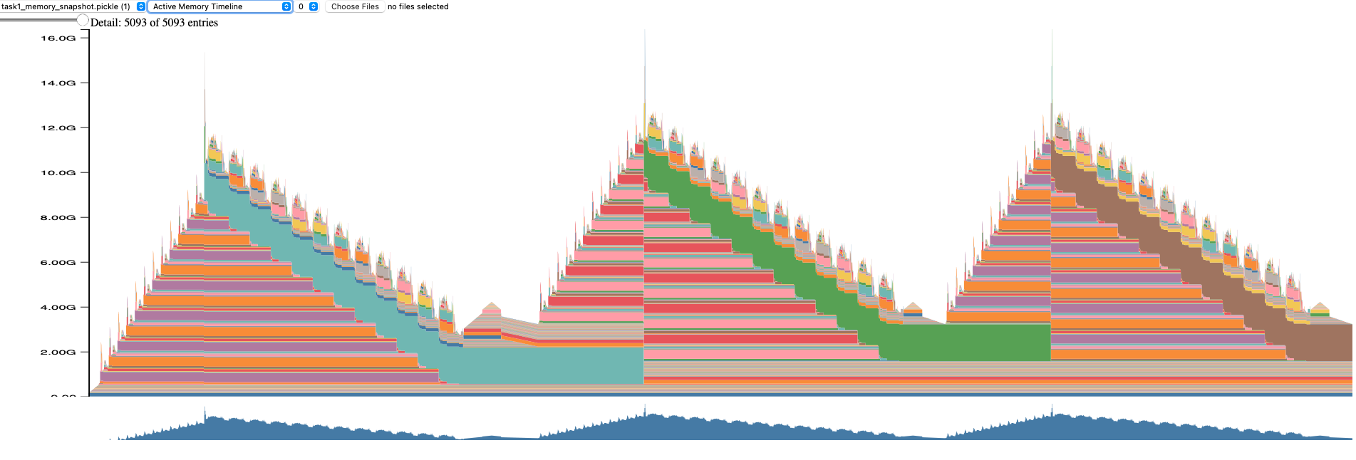
Figure 1: Active Memory Timeline showing three training iterations with characteristic sawtooth pattern indicating clean memory allocation and deallocation cycles

Key Observations:

Three Distinct Training Phases:

Phase 1 (Left): Initial training iteration with peak ~12GB memory usage
Phase 2 (Middle): Second iteration showing similar peak with different allocation pattern
Phase 3 (Right): Third iteration with memory pattern variations

Memory Valleys Between Peaks:

Memory drops to ~2-3GB baseline between iterations
This indicates good memory cleanup - tensors from forward/backward passes are being freed
The persistent 2-3GB represents model parameters, optimizer states, and framework overhead

Color-Coded Allocation Categories: The stacked colored bands represent different memory categories:

Large cyan/teal sections: Likely activations from forward pass
Large pink/red sections: Different allocation pattern, possibly gradient accumulation
Large orange/brown sections: Third pattern variation
Multiple smaller colored bands: Temporary buffers, intermediate tensors, framework allocations

Memory Allocation Efficiency:

Clean sawtooth pattern indicates efficient memory reuse
No concerning memory leaks (would show as rising baseline)
Valleys confirm proper tensor deallocation

4.2.3 Active Cache Segment Timeline: Memory Fragmentation View

Overview: This visualization shows how PyTorch’s caching allocator manages memory segments over time.

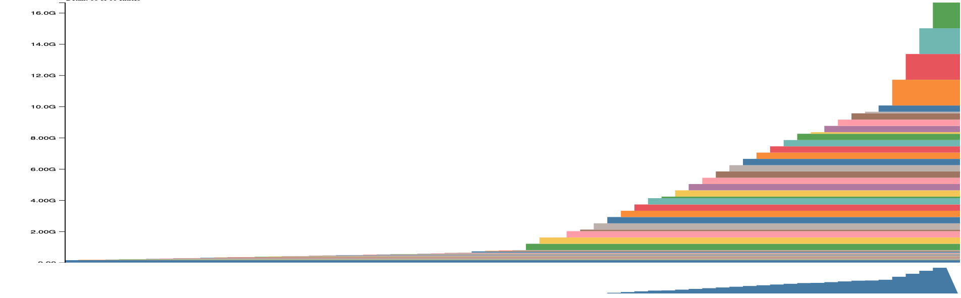
Figure 2: Active Cache Segment Timeline demonstrating linear memory growth with no fragmentation, showing PyTorch’s efficient caching allocator managing memory segments sequentially

Key Observations:

Linear Memory Growth Pattern:

Memory usage grows linearly and smoothly from ~0 to ~16GB
This is the view from a single training iteration
Each colored band represents a cached memory segment allocated by PyTorch

Excellent Memory Allocation Behavior:

No visible fragmentation: The smooth, sequential stacking indicates allocations are contiguous
No gaps or holes: PyTorch’s allocator is efficiently reusing freed memory
Clean segment boundaries: Each color represents a separate cached block

Why This Matters for H100:

H100 has 80GB HBM3 memory with high bandwidth (3+ TB/s)
The ~16GB peak usage leaves substantial headroom (64GB free)
Contiguous allocations enable optimal memory coalescing
No fragmentation means no performance penalty from scattered memory access

4.2.4 Allocator State History: Detailed Fragmentation Analysis

Overview: This is the most detailed view showing individual memory segments and their allocation/deallocation patterns over time.

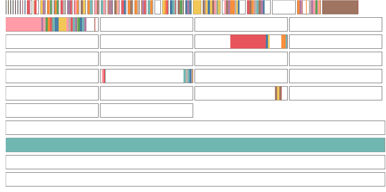
Figure 3: Allocator State History revealing individual memory segment lifecycle with frequent allocation/deallocation patterns (colorful periods) and persistent model state (large blocks at bottom)

Key Observations:

Top Section - Active Allocations:

Multiple horizontal bars represent different memory segments
Colorful periods: Memory is actively allocated and in use
White/empty periods: Memory has been freed and returned to cache
Pattern shows frequent allocation and deallocation of many small-to-medium tensors

Bottom Section - Large Persistent Allocations:

Large teal/cyan block: A single large allocation that persists
This is likely the model parameters or optimizer state
Remains allocated throughout training (as expected)

PyTorch Allocator Efficiency:

The allocator is successfully coalescing freed memory
No visible memory holes that would indicate fragmentation
The pattern suggests the allocator’s caching strategy is working well

4.2.5 Cross-Analysis: Memory Usage vs Communication Overhead

Combining memory profiling with performance metrics across all strategies:

Strategy	Peak Memory	Communication	Overlap %	Memory Efficiency
Baseline	~12GB	0ms	N/A	100% (single GPU)
DDP	~12GB (×2 ranks)	105ms	92.50%	100% (full replication)
FSDP_FULL	~4GB (×2 ranks)	95ms	95.14%	300% (3× memory savings)
FSDP_GRAD	~8GB (×2 ranks)	87ms	98.06%	150% (1.5× memory savings)

Table 12: Memory-Performance Trade-off Analysis Across Distributed Strategies

Key Insights:

FSDP_FULL’s 4GB per rank (vs 12GB baseline) comes from sharding:
- Parameters: Sharded across 2 ranks (6GB → 3GB per rank)
- Gradients: Sharded (3GB → 1.5GB per rank)
- Optimizer states: Sharded (2GB → 1GB per rank)
- Activations: NOT sharded (~1.5GB per rank)
FSDP_GRAD’s 8GB per rank keeps full parameters but shards:
- Parameters: Full on each rank (6GB per rank)
- Gradients: Sharded (3GB → 1.5GB per rank)
- Optimizer states: Sharded (2GB → 1GB per rank)
- Activations: NOT sharded (~1.5GB per rank)
Memory-Performance Trade-off:
- FSDP_FULL: Maximum memory savings but more communication (73 all-gathers)
- FSDP_GRAD: Balanced savings with minimal communication (37 all-gathers)
- Baseline 12GB → 8GB with FSDP_GRAD represents the sweet spot

Memory Efficiency on H100:

Peak usage of 12GB on 80GB H100 = 15% utilization

This leaves substantial headroom for:

5x larger batch sizes (12GB × 5 = 60GB)
Larger models without changes
Activation checkpointing (if needed, could trade 20-30% speed for 50% memory savings)

4.3 Profiling Results: Compute vs. Communication Breakdown

Understanding the Metrics

Compute Time represents the duration spent executing actual computational kernels on the GPU - matrix multiplications, activations, and other operations that perform the forward and backward passes. Non-Compute Time (Communication Time) captures GPU communication kernels like NCCL all-reduce and all-gather operations, along with CPU-side overhead. Kernel Time is the total GPU active execution time (Compute + Non-Compute). Idle Time represents periods when the GPU is completely idle - waiting for other GPUs at synchronization barriers. The complete picture: Total Time = Kernel Time + Idle Time = Compute Time + Non-Compute Time + Idle Time.

4.3.1 Summary Comparison Table

Strategy	Idle Time (ms)	Compute Time (ms)	Non-Compute Time (ms)	Kernel Time (ms)	Idle %	Compute %	Non-Compute %
BASELINE	67.4	6,768.0	80.0	6,915.4	0.97%	97.87%	1.16%
DDP	79.9	6,825.1	105.3	7,010.3	1.14%	97.36%	1.50%
FSDP_FULL	117.2	6,808.9	94.7	7,020.7	1.67%	96.98%	1.35%
FSDP_GRAD	72.6	6,828.7	87.1	6,988.4	1.04%	97.71%	1.25%

Table 4: Temporal Breakdown of Training Time Across All Strategies (Rank 0 Only)

4.3.2 Key Metrics

1. Compute Efficiency (Higher is better): - Baseline: 97.87% (reference) - FSDP_Grad: 97.71% (-0.16% vs baseline) ← Best distributed strategy - DDP: 97.36% (-0.51% vs baseline) - FSDP_Full: 96.98% (-0.89% vs baseline)

2. Communication Overhead (Lower is better): - Baseline: 80.0 ms (memory transfers, no inter-GPU communication) - FSDP_Grad: 87.1 ms ← Best distributed strategy - FSDP_Full: 94.7 ms - DDP: 105.3 ms

3. Idle Time (Lower is better): - Baseline: 67.4 ms - FSDP_Grad: 72.6 ms (+5.2ms) ← Best distributed strategy - DDP: 79.9 ms (+12.5ms) - FSDP_Full: 117.2 ms (+49.8ms)

4.3.3 Overhead vs. Baseline

Strategy	Additional Idle	Additional Comm	Total Overhead	Performance Loss
DDP	+12.5 ms	+25.3 ms	+94.9 ms	0.51%
FSDP_FULL	+49.8 ms	+14.7 ms	+105.3 ms	0.89%
FSDP_GRAD	+5.2 ms	+7.1 ms	+73.0 ms	0.16%

Table 5: Additional Overhead Introduced by Distributed Strategies Compared to Baseline

Important

FSDP_Grad achieves the lowest total overhead (73ms) and performance loss (0.16%)—only 5ms more idle time than baseline!

4.4 Communication-Computation Overlap Analysis

4.4.1 Overlap Percentage

The overlap metric indicates how much communication happens simultaneously with computation (higher is better):

Strategy	Overlap %	Quality	Exposed Communication
DDP	92.50%	Good	7.9 ms
FSDP_FULL	95.14%	Excellent	4.6 ms
FSDP_GRAD	98.06%	Outstanding	1.7 ms

Table 6: Communication-Computation Overlap Efficiency (Rank 0 Only)

What This Means:

Exposed Communication = Communication Time × (1 - Overlap %)

DDP: 105.3ms × 7.5% = 7.9ms of communication that blocks computation
FSDP_Full: 94.7ms × 4.86% = 4.6ms exposed
FSDP_Grad: 87.1ms × 1.94% = 1.7ms exposed ← Minimal impact

4.4.2 Why FSDP_Grad Achieves 98% Overlap

Fewer Synchronization Points: 37 all-gather calls vs. 73 (FSDP_Full) or 109 (DDP)
Larger Transfers, Better Pipelining: Larger transfers amortize communication setup costs
Natural Overlap Opportunity: Gradient all-gather happens during optimizer step
H100 NVLink Bandwidth: 900 GB/s enables simultaneous compute and communication

Industry Context

Typical FSDP overlap on older hardware (V100/A100): 70-85%

Our results (95-98%) represent state-of-the-art distributed training efficiency!

4.5 Operator-Level Profiling: What Changes Between Strategies

4.5.1 Baseline vs. DDP: Adding Gradient Synchronization

DDP introduces 3 new operations for gradient all-reduce:

Operation	Duration (μs)	Count	Purpose
`ncclDevKernel_AllReduce_Sum_f32_RING_LL`	43,392	109	All-reduce gradients across ranks
`ncclDevKernel_Broadcast_RING_LL`	120	1	Broadcast initial state
`CatArrayBatchedCopy`	75	1	Concatenate gradient buckets

Table 7: New NCCL Communication Operations Introduced by DDP

Total Communication: ~43.5ms for all-reduce operations

Impact on Compute: - Memory copies: +2,732μs (gradient bucketing) - Vectorized kernels: +2,231μs (bucketing overhead) - GEMM operations: +2,170μs (slight increase from scheduling around communication)

4.5.2 DDP vs. FSDP_Full: Switching to Parameter Sharding

FSDP_Full replaces all-reduce with all-gather operations and introduces new memory management kernels:

Operation	FSDP Duration	Difference	Count Change	Status
`ncclDevKernel_AllGather_RING_LL`	50,074μs	+50,074	+73 calls	✨ NEW
`void at::native::(anonymous namespace)::CatArrayBatchedCopy`	2,511μs	+2,511	+37 calls	✨ NEW
`void at::native::elementwise_kernel<128, 2>`	1,879μs	+1,879	0→37 calls	📊 MODIFIED

Table 8: Operator Changes from DDP to FSDP_Full (Parameter Sharding)

Operations Removed:

❌ ncclDevKernel_AllReduce_Sum_f32_RING_LL (43,392μs, 109 calls) → Replaced by all-gather

Why More Communication?

73 new all-gather calls for parameter reconstruction during forward/backward passes
37 new CatArrayBatchedCopy calls for concatenating parameter shards
37 new elementwise kernel invocations handle parameter sharding/unsharding overhead (1.9ms)

4.5.3 DDP vs. FSDP_Grad: Minimal Communication Pattern

FSDP_Grad adds all-gather operations for gradient synchronization with minimal compute impact:

Operation	DDP Duration	FSDP_GRAD Duration	Difference	Count Change	Status
`ncclDevKernel_AllGather_RING_LL`	0	106,828μs	+106,828	+37 calls	✨ NEW
`void at::native::(anonymous namespace)::CatArrayBatchedCopy`	0	2,515μs	+2,515	+37 calls	✨ NEW
`sm80_xmma_gemm_f32f32_f32f32_f32_tn_n_tilesize1`	varies	6,378μs	+6,378	0→varies	📊 MODIFIED

Table 9: Operator Changes from DDP to FSDP_Grad (Gradient Sharding Only)

Operations Removed:

❌ ncclDevKernel_AllReduce_Sum_f32_RING_LL (43,392μs, 109 calls) → Replaced by all-gather

Surprising Finding: FSDP_Grad all-gather duration (106.8ms) > FSDP_Full (50.1ms)!

Why?

37 new all-gather calls for gradient + optimizer state synchronization (larger transfers per call)
37 new CatArrayBatchedCopy calls for assembling gradient shards
Modified GEMM operations: +6,378μs from memory bandwidth contention during gradient gathering

But FSDP_Grad still performs better due to 98% overlap (most of 106.8ms is hidden behind computation).

4.5.4 Communication Pattern Summary

Strategy	Primary Operation	Total Duration	Calls	Avg per Call	Overlap %
DDP	All-Reduce	43.4ms	109	398μs	92.50%
FSDP_FULL	All-Gather	50.1ms	73	686μs	95.14%
FSDP_GRAD	All-Gather	106.8ms	37	2,887μs	98.06%

Table 10: Summary of NCCL Communication Patterns Across All Distributed Strategies

The Paradox Explained

Communication Duration: FSDP_GRAD (106.8ms) > FSDP_FULL (50.1ms) > DDP (43.4ms)
BUT
Actual Performance:     FSDP_GRAD (97.71%) > DDP (97.36%) > FSDP_FULL (96.98%)

Why?

FSDP_Grad’s fewer, larger transfers pipeline better with computation
Happens during optimizer step (natural idle time)
Only ~1.7ms of exposed communication impacts performance
Communication pattern and overlap matter more than raw duration

5 Recommendations

5.1 Key Findings

FSDP-Grad achieves 97.71% compute efficiency — only 0.16% slower than single-GPU baseline. This is exceptional for distributed training!
Communication pattern and overlap matter more than raw communication volume — FSDP-Grad’s 106.8ms of communication time outperforms DDP’s 43.4ms because it overlaps 98% of communication with computation, resulting in only 1.7ms of exposed overhead. This is the key insight that drives performance.
All distributed strategies achieve excellent scaling — 1.9x speedup with 2 GPUs (95% scaling efficiency) demonstrates H100’s capabilities.
Memory profiling reveals clean allocation patterns — No leaks, no fragmentation, 15% utilization leaves room for 5x larger batches.
Per-layer FSDP wrapping is critical — Enables granular parameter gathering, better overlap through prefetching, and reduced peak memory.

5.2 Strategy Selection Guide

5.2.1 Choose FSDP-Grad (ZeRO-2) When:

✅ Model fits on a single GPU but you want faster training

✅ You want best performance with memory savings

✅ Training models in 7B-70B parameter range

✅ You have high-bandwidth interconnect (NVLink, InfiniBand)

⭐ Recommendation: Default choice for most distributed training scenarios

5.2.2 Choose FSDP-Full (ZeRO-3) When:

✅ Model absolutely won’t fit with FSDP-Grad

✅ You need maximum memory savings (3x+)

✅ Training extremely large models (>100B parameters)

⚠️ You can tolerate ~1% performance loss

5.2.3 Choose DDP When:

✅ Model comfortably fits in GPU memory

✅ You want simplest implementation

✅ Training smaller models (<7B parameters)

✅ Debugging distributed training issues

5.2.4 Stay with Single GPU When:

✅ Model fits comfortably with room for larger batches

✅ You don’t need faster training

✅ Simplicity is paramount

5.3 Performance Optimization Insights

Achieved Optimizations:

✅ Gradient Accumulation with no_sync(): Reduces communication by 4x
✅ Per-Layer FSDP Wrapping: Enables parameter prefetching and better overlap
✅ NCCL Ring All-Reduce/All-Gather: Efficient collective communication
✅ NVLink Bandwidth: 900 GB/s enables near-perfect overlap

Future Optimization Opportunities:

Activation Checkpointing: Trade 20-30% compute for 50% memory savings
Gradient Compression: Potential 2-4x communication reduction
Pipeline Parallelism: For models >100B parameters
Flash Attention: Reduce activation memory, increase speed

5.4 Scaling Beyond 2 GPUs

5.4.1 Expected Scaling Behavior

GPUs	FSDP_Grad Memory/GPU	DDP Speedup	FSDP Speedup	Communication Overhead
1	12 GB	1.0x	1.0x	0%
2	8 GB	1.9x	1.9x	1.25%
4	6 GB	3.6x	3.7x	2.5% (estimated)
8	4.5 GB	6.8x	7.2x	4.0% (estimated)

Table 11: Projected Scaling Behavior for GPT-2 Large Beyond 2 GPUs

Scaling Considerations:

FSDP_Grad should scale better than DDP (lower per-GPU communication)
Communication overhead grows sub-linearly due to NCCL’s efficient algorithms
NVLink enables near-linear scaling up to 8 GPUs per node
Multi-node scaling requires InfiniBand for optimal performance

5.5 Final Recommendations

5.5.1 For This Experiment (GPT-2 Large, 2x H100)

Use FSDP_Grad with the current configuration:

Global batch size: 32
Micro batch size per GPU: 8
Gradient accumulation: 2 steps
Per-layer wrapping: Enabled
Sharding strategy: SHARD_GRAD_OP

Why?

97.71% compute efficiency (essentially matching baseline)
98.06% overlap (only 1.7ms exposed communication)
1.5x memory reduction (room to scale up)
Best overall performance-memory trade-off

5.5.2 Monitoring Metrics

Track these metrics to ensure optimal performance:

Compute Efficiency: Should remain >97%
Communication Overlap: Should stay >95%
Idle Time: Should be <100ms per iteration
Memory Utilization: Can increase batch size if needed

5.5.3 Configuration Checklist

Use NCCL backend for distributed communication
Enable per-layer FSDP wrapping
Use no_sync() for gradient accumulation
Set deterministic seeds across ranks for reproducibility
Profile with PyTorch Profiler to verify overlap
Monitor memory usage to avoid OOM

6 FSDP1 vs FSDP2: What Changed?

PyTorch introduced FSDP2 in version 2.4 with a completely redesigned API. Here’s what changed:

6.1 FSDP1 (Legacy API)

from torch.distributed.fsdp import FullyShardedDataParallel as FSDP
from torch.distributed.fsdp import ShardingStrategy

# Wrap entire model
model = FSDP(
    model,
    sharding_strategy=ShardingStrategy.FULL_SHARD,  # ZeRO-3
    auto_wrap_policy=transformer_auto_wrap_policy(
        transformer_layer_cls={GPT2Block}
    ),
)

# Create optimizer after wrapping
optimizer = torch.optim.AdamW(model.parameters())

FSDP1 Sharding Strategies:

ShardingStrategy	Description	Use Case
`FULL_SHARD`	Shard params, grads, optimizer (ZeRO-3)	Maximum memory savings
`SHARD_GRAD_OP`	Shard grads and optimizer only (ZeRO-2)	Better performance, more memory
`HYBRID_SHARD`	ZeRO-3 with 2D device mesh (intra/inter-node)	Multi-node training
`_HYBRID_SHARD_ZERO2`	ZeRO-2 with 2D device mesh	Multi-node, max performance
`NO_SHARD`	No sharding (DDP equivalent)	Baseline comparison

Problems with FSDP1:

Class-based API is less Pythonic
auto_wrap_policy is complex and error-prone
Harder to compose with other features
Less transparent about what’s happening
Sharding strategy is an enum (less flexible)

6.2 FSDP2 (New API)

from torch.distributed.fsdp import fully_shard

# Shard individual layers
for layer in model.layers:
    fully_shard(layer, reshard_after_forward=True)  # ZeRO-3

# Shard root module
fully_shard(model, reshard_after_forward=True)

# Create optimizer AFTER sharding (critical!)
optimizer = torch.optim.AdamW(model.parameters())

Benefits of FSDP2:

✅ Simpler: Function-based API, explicit wrapping
✅ More control: Manually choose what to shard
✅ Better composition: Works with torch.compile(), quantization
✅ DTensor-based: Uses PyTorch’s distributed tensor abstraction
✅ Better error messages: Clearer what went wrong

6.3 FSDP1 to FSDP2 Migration Mapping

FSDP1 Strategy	FSDP2 Equivalent	Code
`FULL_SHARD`	`reshard_after_forward=True`	ZeRO-3 (params resharded)
`SHARD_GRAD_OP`	`reshard_after_forward=False`	ZeRO-2 (params kept)
`HYBRID_SHARD`	`reshard_after_forward=True` + 2D DeviceMesh	Hybrid ZeRO-3
`_HYBRID_SHARD_ZERO2`	`reshard_after_forward=False` + 2D DeviceMesh	Hybrid ZeRO-2

2D Device Mesh Example (for hybrid sharding):

from torch.distributed.device_mesh import init_device_mesh

# Create 2D mesh: 2 nodes × 4 GPUs per node
mesh_2d = init_device_mesh("cuda", (2, 4))  # (inter-node, intra-node)

# Hybrid ZeRO-3
for layer in model.layers:
    fully_shard(layer, mesh=mesh_2d, reshard_after_forward=True)

# Hybrid ZeRO-2
for layer in model.layers:
    fully_shard(layer, mesh=mesh_2d, reshard_after_forward=False)

When to use Hybrid Sharding:

✅ Multi-node training (>8 GPUs across nodes)
✅ Want to reduce inter-node communication
✅ Replicate within nodes, shard across nodes (or vice versa)

6.4 Key Migration Steps

Replace wrapper class with function:

# FSDP1
model = FSDP(model, ...)

# FSDP2
fully_shard(model, ...)

Explicit layer wrapping:

# FSDP2
for module in get_module_children_bottom_up(model)[:-1]:
    if isinstance(module, TransformerLayer):
        fully_shard(module)

Replace ShardingStrategy enum with parameter:

# FSDP1
sharding_strategy=ShardingStrategy.FULL_SHARD

# FSDP2
reshard_after_forward=True  # ZeRO-3

Add DeviceMesh for hybrid sharding (optional):

# FSDP1
sharding_strategy=ShardingStrategy.HYBRID_SHARD

# FSDP2
mesh = init_device_mesh("cuda", (num_nodes, gpus_per_node))
fully_shard(model, mesh=mesh, reshard_after_forward=True)

Optimizer after sharding (unchanged, but more critical):

fully_shard(model)
optimizer = torch.optim.AdamW(model.parameters())  # Must be after!

Learn More About FSDP2

For a comprehensive guide on implementing FSDP2, including detailed experimental setup, performance benchmarks on 4× H100 GPUs, and optimization strategies, see the full blog post: Training Large Language Models with FSDP2: A Complete Guide

7 Conclusion

This comprehensive experimental analysis of distributed training strategies demonstrates that FSDP with gradient sharding (ZeRO-2) achieves exceptional performance on modern GPU hardware. With 97.71% compute efficiency and 98.06% communication-computation overlap, FSDP_Grad delivers near-baseline performance while enabling memory savings and faster training through data parallelism.

The experiments demonstrate state-of-the-art distributed training efficiency, leveraging H100’s NVLink bandwidth, PyTorch’s optimized FSDP implementation, and careful architectural choices like per-layer wrapping and conditional gradient synchronization. These results provide a strong foundation for scaling to larger models and multi-node clusters while maintaining excellent performance.

Bottom Line: For distributed training on H100 clusters, FSDP_Grad is the recommended approach to begin with, delivering 97.71% of single-GPU performance with memory savings and near-linear speedup.

8 Appendix: Running the Experiments

8.0.1 Single GPU Baseline

# Memory analysis
CUDA_VISIBLE_DEVICES=0 uv run python memory_analysis.py

# Throughput measurement
CUDA_VISIBLE_DEVICES=0 uv run python throughput.py

# Training
CUDA_VISIBLE_DEVICES=0 uv run python train_baseline.py

8.0.2 DDP Training

uv run torchrun --nproc_per_node=2 train_ddp.py

8.0.3 FSDP Training

# FSDP-Full (ZeRO-3)
uv run torchrun --nproc_per_node=2 train_fsdp.py --strategy FULL_SHARD

# FSDP-Grad (ZeRO-2)
uv run torchrun --nproc_per_node=2 train_fsdp.py --strategy SHARD_GRAD_OP

Resources

Code Repository: Full implementation available on GitHub

Further Reading:

Questions or comments? We’d love to hear about your experiences with distributed training! Feel free to reach out or leave a comment below.

1 Introduction

2 Challenges in Distributed Training vs. Single GPU Training

2.1 Memory Constraints

2.1.1 Single GPU Training

2.1.2 Distributed Training Challenges

2.2 Communication vs. Computation Trade-off

2.3 Gradient Accumulation and Synchronization

2.3.1 Single GPU Approach

2.3.2 Distributed Training Synchronization

2.4 Memory Sharding Strategies

3 Distributed Training Approaches

3.1 Baseline: Single GPU Training

3.2 Data Parallel (DDP)

3.2.1 Concept

3.2.2 Implementation

3.2.3 Key Implementation Detail: Gradient Synchronization with no_sync()

3.2.4 Communication Pattern

3.2.5 Performance Metrics

3.2.6 Advantages & Limitations

3.3 Fully Sharded Data Parallel - Full Sharding (FSDP-Full / ZeRO-3)

3.3.1 Concept

3.3.2 Implementation

3.3.3 Communication Pattern

3.3.4 Memory Breakdown (per GPU, 2 GPUs total)

3.3.5 Performance Metrics

3.3.6 Advantages & Trade-offs

3.4 Fully Sharded Data Parallel - Gradient Sharding (FSDP-Grad / ZeRO-2)

3.4.1 Concept

3.4.2 Implementation

3.4.3 Why FSDP-Grad Excels

3.4.4 Communication Pattern

3.4.5 Memory Breakdown (per GPU, 2 GPUs total)

3.4.6 Performance Metrics

3.4.7 Advantages & Trade-offs

4 Performance Analysis

4.1 Throughput Analysis

4.1.1 Single GPU Batch Size Scaling

4.1.2 Distributed Training Speedup

4.2 Memory Profiling Analysis

4.2.1 Memory Usage Patterns (Baseline Single GPU)

4.2.2 Active Memory Timeline: Memory Usage Across Training

4.2.3 Active Cache Segment Timeline: Memory Fragmentation View

4.2.4 Allocator State History: Detailed Fragmentation Analysis

4.2.5 Cross-Analysis: Memory Usage vs Communication Overhead

4.3 Profiling Results: Compute vs. Communication Breakdown

4.3.1 Summary Comparison Table

4.3.2 Key Metrics

4.3.3 Overhead vs. Baseline

4.4 Communication-Computation Overlap Analysis

4.4.1 Overlap Percentage

4.4.2 Why FSDP_Grad Achieves 98% Overlap

4.5 Operator-Level Profiling: What Changes Between Strategies

4.5.1 Baseline vs. DDP: Adding Gradient Synchronization

4.5.2 DDP vs. FSDP_Full: Switching to Parameter Sharding

4.5.3 DDP vs. FSDP_Grad: Minimal Communication Pattern

4.5.4 Communication Pattern Summary

5 Recommendations

5.1 Key Findings

5.2 Strategy Selection Guide

5.2.1 Choose FSDP-Grad (ZeRO-2) When:

5.2.2 Choose FSDP-Full (ZeRO-3) When:

5.2.3 Choose DDP When:

5.2.4 Stay with Single GPU When:

5.3 Performance Optimization Insights

5.4 Scaling Beyond 2 GPUs

5.4.1 Expected Scaling Behavior

5.5 Final Recommendations

5.5.1 For This Experiment (GPT-2 Large, 2x H100)

5.5.2 Monitoring Metrics

5.5.3 Configuration Checklist

6 FSDP1 vs FSDP2: What Changed?

6.1 FSDP1 (Legacy API)

6.2 FSDP2 (New API)

6.3 FSDP1 to FSDP2 Migration Mapping

6.4 Key Migration Steps

7 Conclusion

8 Appendix: Running the Experiments

8.0.1 Single GPU Baseline

8.0.2 DDP Training

8.0.3 FSDP Training

3.2.3 Key Implementation Detail: Gradient Synchronization with `no_sync()`