from importlib.metadata import version

print("torch version:", version("torch"))
torch version: 2.4.0Packages that are being used in this notebook:
In [1]:
from importlib.metadata import version
print("torch version:", version("torch"))torch version: 2.4.0

In [2]:
import torch

inputs = torch.tensor(
  [[0.43, 0.15, 0.89], # Your     (x^1)
   [0.55, 0.87, 0.66], # journey  (x^2)
   [0.57, 0.85, 0.64], # starts   (x^3)
   [0.22, 0.58, 0.33], # with     (x^4)
   [0.77, 0.25, 0.10], # one      (x^5)
   [0.05, 0.80, 0.55]] # step     (x^6)
)
(In this book, we follow the common machine learning and deep learning convention where training examples are represented as rows and feature values as columns; in the case of the tensor shown above, each row represents a word, and each column represents an embedding dimension)
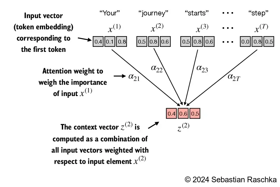
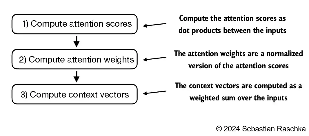
The primary objective of this section is to demonstrate how the context vector \(z^{(2)}\) is calculated using the second input sequence, \(x^{(2)}\), as a query
The figure depicts the initial step in this process, which involves calculating the attention scores ω between \(x^{(2)}\) and all other input elements through a dot product operation

In [3]:
query = inputs[1]  # 2nd input token is the query

attn_scores_2 = torch.empty(inputs.shape[0])
for i, x_i in enumerate(inputs):
    attn_scores_2[i] = torch.dot(x_i, query) # dot product (transpose not necessary here since they are 1-dim vectors)

print(attn_scores_2)
tensor([0.9544, 1.4950, 1.4754, 0.8434, 0.7070, 1.0865])In [4]:
res = 0.

for idx, element in enumerate(inputs[0]):
    res += inputs[0][idx] * query[idx]

print(res)
print(torch.dot(inputs[0], query))
tensor(0.9544)
tensor(0.9544)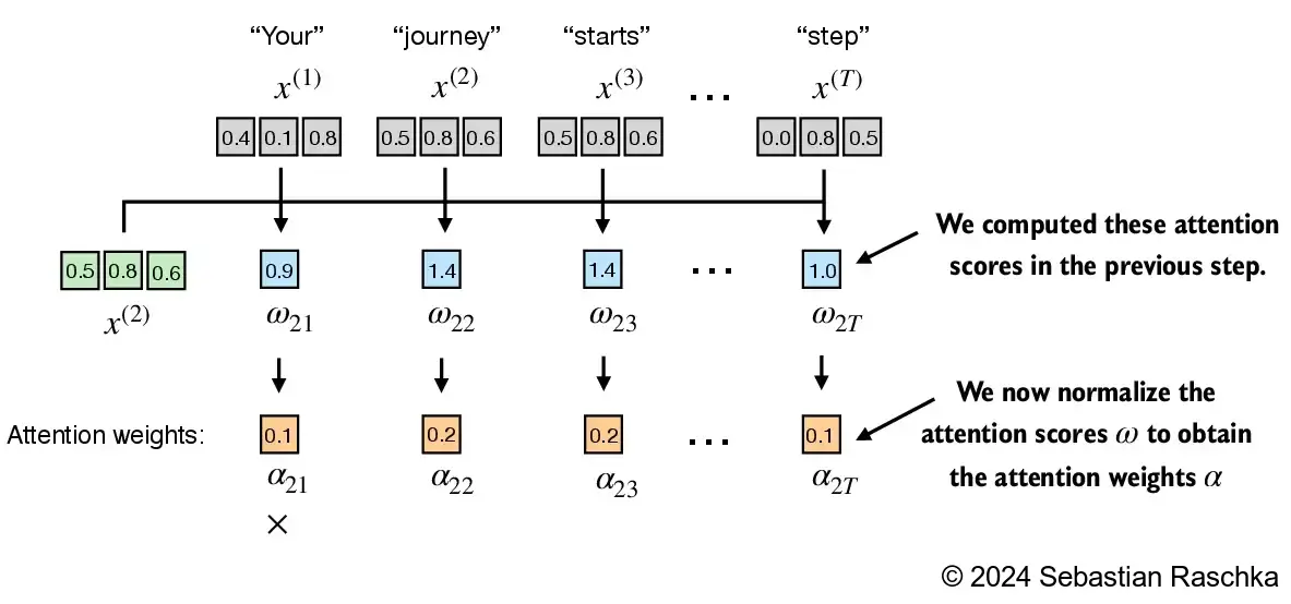
In [5]:
attn_weights_2_tmp = attn_scores_2 / attn_scores_2.sum()

print("Attention weights:", attn_weights_2_tmp)
print("Sum:", attn_weights_2_tmp.sum())
Attention weights: tensor([0.1455, 0.2278, 0.2249, 0.1285, 0.1077, 0.1656])
Sum: tensor(1.0000)In [6]:
def softmax_naive(x):
    return torch.exp(x) / torch.exp(x).sum(dim=0)

attn_weights_2_naive = softmax_naive(attn_scores_2)

print("Attention weights:", attn_weights_2_naive)
print("Sum:", attn_weights_2_naive.sum())
Attention weights: tensor([0.1385, 0.2379, 0.2333, 0.1240, 0.1082, 0.1581])
Sum: tensor(1.)In [7]:
attn_weights_2 = torch.softmax(attn_scores_2, dim=0)

print("Attention weights:", attn_weights_2)
print("Sum:", attn_weights_2.sum())
Attention weights: tensor([0.1385, 0.2379, 0.2333, 0.1240, 0.1082, 0.1581])
Sum: tensor(1.)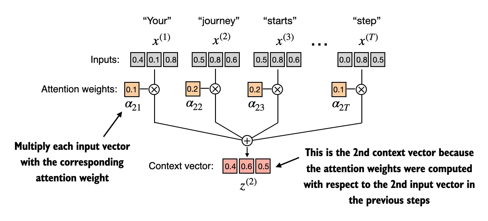
In [8]:
query = inputs[1] # 2nd input token is the query

context_vec_2 = torch.zeros(query.shape)
for i,x_i in enumerate(inputs):
    context_vec_2 += attn_weights_2[i]*x_i

print(context_vec_2)
tensor([0.4419, 0.6515, 0.5683])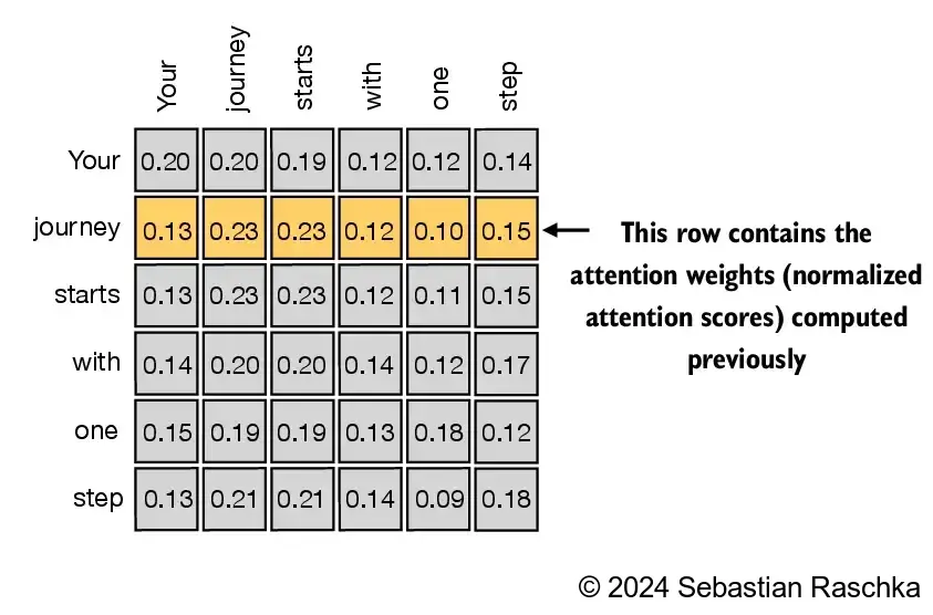
In [9]:
attn_scores = torch.empty(6, 6)

for i, x_i in enumerate(inputs):
    for j, x_j in enumerate(inputs):
        attn_scores[i, j] = torch.dot(x_i, x_j)

print(attn_scores)
tensor([[0.9995, 0.9544, 0.9422, 0.4753, 0.4576, 0.6310],
[0.9544, 1.4950, 1.4754, 0.8434, 0.7070, 1.0865],
[0.9422, 1.4754, 1.4570, 0.8296, 0.7154, 1.0605],
[0.4753, 0.8434, 0.8296, 0.4937, 0.3474, 0.6565],
[0.4576, 0.7070, 0.7154, 0.3474, 0.6654, 0.2935],
[0.6310, 1.0865, 1.0605, 0.6565, 0.2935, 0.9450]])In [10]:
attn_scores = inputs @ inputs.T
print(attn_scores)
tensor([[0.9995, 0.9544, 0.9422, 0.4753, 0.4576, 0.6310],
[0.9544, 1.4950, 1.4754, 0.8434, 0.7070, 1.0865],
[0.9422, 1.4754, 1.4570, 0.8296, 0.7154, 1.0605],
[0.4753, 0.8434, 0.8296, 0.4937, 0.3474, 0.6565],
[0.4576, 0.7070, 0.7154, 0.3474, 0.6654, 0.2935],
[0.6310, 1.0865, 1.0605, 0.6565, 0.2935, 0.9450]])In [11]:
attn_weights = torch.softmax(attn_scores, dim=-1)
print(attn_weights)
tensor([[0.2098, 0.2006, 0.1981, 0.1242, 0.1220, 0.1452],
[0.1385, 0.2379, 0.2333, 0.1240, 0.1082, 0.1581],
[0.1390, 0.2369, 0.2326, 0.1242, 0.1108, 0.1565],
[0.1435, 0.2074, 0.2046, 0.1462, 0.1263, 0.1720],
[0.1526, 0.1958, 0.1975, 0.1367, 0.1879, 0.1295],
[0.1385, 0.2184, 0.2128, 0.1420, 0.0988, 0.1896]])In [12]:
row_2_sum = sum([0.1385, 0.2379, 0.2333, 0.1240, 0.1082, 0.1581])
print("Row 2 sum:", row_2_sum)

print("All row sums:", attn_weights.sum(dim=-1))
Row 2 sum: 1.0
All row sums: tensor([1.0000, 1.0000, 1.0000, 1.0000, 1.0000, 1.0000])In [13]:
all_context_vecs = attn_weights @ inputs
print(all_context_vecs)
tensor([[0.4421, 0.5931, 0.5790],
[0.4419, 0.6515, 0.5683],
[0.4431, 0.6496, 0.5671],
[0.4304, 0.6298, 0.5510],
[0.4671, 0.5910, 0.5266],
[0.4177, 0.6503, 0.5645]])In [14]:
print("Previous 2nd context vector:", context_vec_2)Previous 2nd context vector: tensor([0.4419, 0.6515, 0.5683])
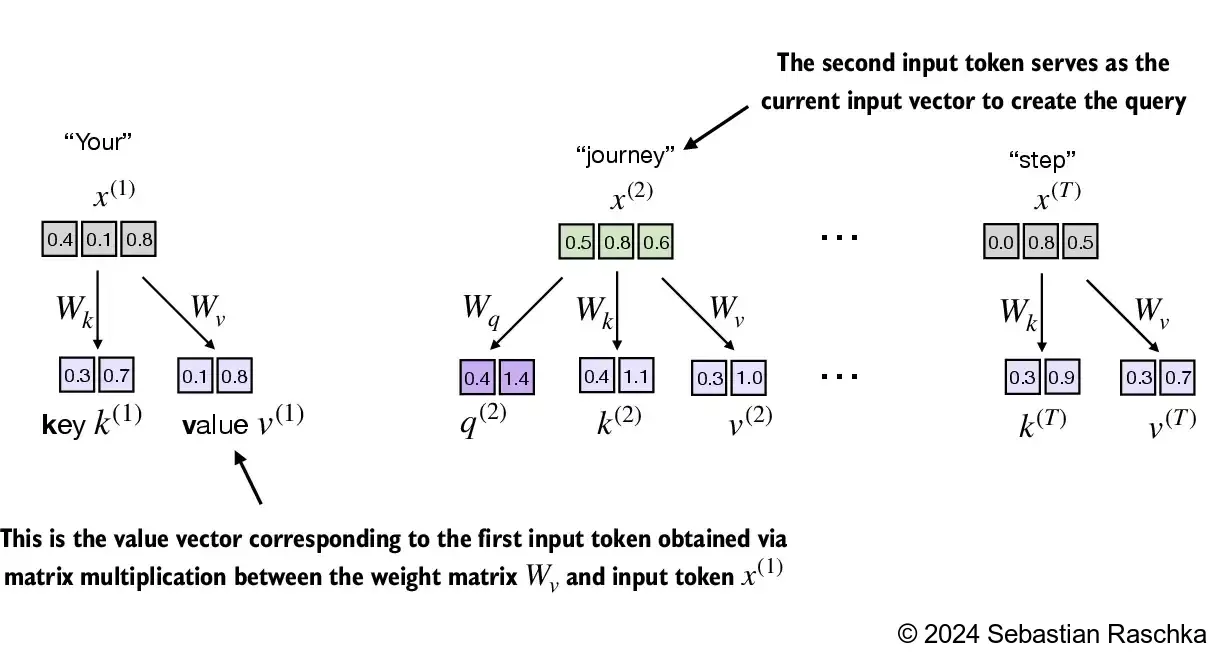
Implementing the self-attention mechanism step by step, we will start by introducing the three training weight matrices \(W_q\), \(W_k\), and \(W_v\)
These three matrices are used to project the embedded input tokens, \(x^{(i)}\), into query, key, and value vectors via matrix multiplication:
In [15]:
x_2 = inputs[1] # second input element
d_in = inputs.shape[1] # the input embedding size, d=3
d_out = 2 # the output embedding size, d=2requires_grad=False to reduce clutter in the outputs for illustration purposes, but if we were to use the weight matrices for model training, we would set requires_grad=True to update these matrices during model trainingIn [16]:
torch.manual_seed(123)

W_query = torch.nn.Parameter(torch.rand(d_in, d_out), requires_grad=False)
W_key   = torch.nn.Parameter(torch.rand(d_in, d_out), requires_grad=False)
W_value = torch.nn.Parameter(torch.rand(d_in, d_out), requires_grad=False)In [17]:
query_2 = x_2 @ W_query # _2 because it's with respect to the 2nd input element
key_2 = x_2 @ W_key
value_2 = x_2 @ W_value

print(query_2)
tensor([0.4306, 1.4551])In [18]:
keys = inputs @ W_key
values = inputs @ W_value

print("keys.shape:", keys.shape)
print("values.shape:", values.shape)
keys.shape: torch.Size([6, 2])
values.shape: torch.Size([6, 2])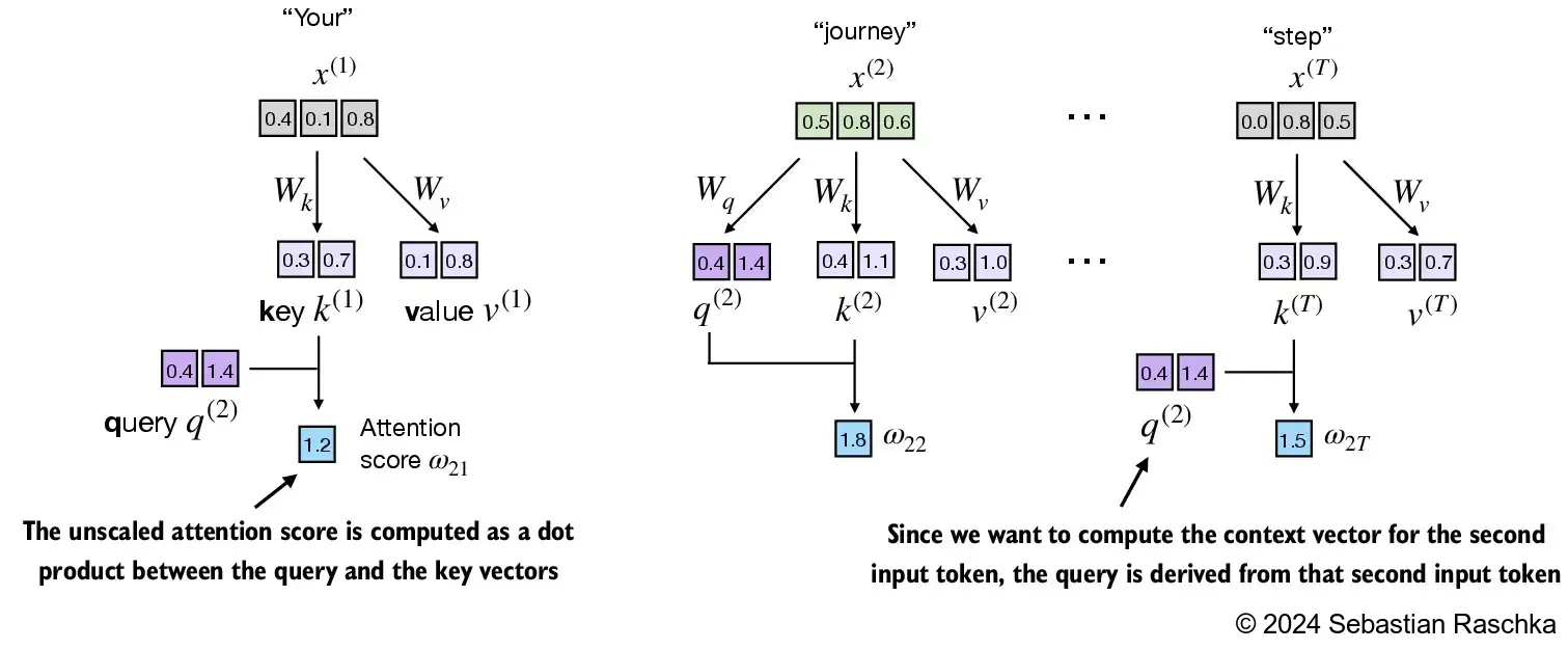
In [19]:
keys_2 = keys[1] # Python starts index at 0
attn_score_22 = query_2.dot(keys_2)
print(attn_score_22)tensor(1.8524)In [20]:
attn_scores_2 = query_2 @ keys.T # All attention scores for given query
print(attn_scores_2)
tensor([1.2705, 1.8524, 1.8111, 1.0795, 0.5577, 1.5440])
d_k**0.5):In [21]:
d_k = keys.shape[1]
attn_weights_2 = torch.softmax(attn_scores_2 / d_k**0.5, dim=-1)
print(attn_weights_2)
tensor([0.1500, 0.2264, 0.2199, 0.1311, 0.0906, 0.1820])
In [22]:
context_vec_2 = attn_weights_2 @ values
print(context_vec_2)
tensor([0.3061, 0.8210])In [23]:
import torch.nn as nn

class SelfAttention_v1(nn.Module):

    def __init__(self, d_in, d_out):
        super().__init__()
        self.W_query = nn.Parameter(torch.rand(d_in, d_out))
        self.W_key   = nn.Parameter(torch.rand(d_in, d_out))
        self.W_value = nn.Parameter(torch.rand(d_in, d_out))

    def forward(self, x):
        keys = x @ self.W_key
        queries = x @ self.W_query
        values = x @ self.W_value

        attn_scores = queries @ keys.T # omega
        attn_weights = torch.softmax(
            attn_scores / keys.shape[-1]**0.5, dim=-1
        )

        context_vec = attn_weights @ values
        return context_vec

torch.manual_seed(123)
sa_v1 = SelfAttention_v1(d_in, d_out)
print(sa_v1(inputs))
tensor([[0.2996, 0.8053],
[0.3061, 0.8210],
[0.3058, 0.8203],
[0.2948, 0.7939],
[0.2927, 0.7891],
[0.2990, 0.8040]], grad_fn=<MmBackward0>)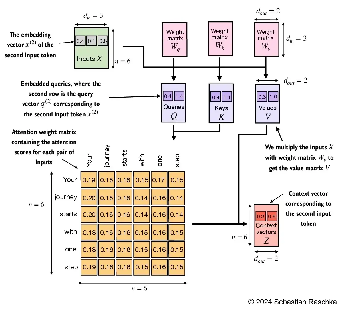
nn.Linear over our manual nn.Parameter(torch.rand(...) approach is that nn.Linear has a preferred weight initialization scheme, which leads to more stable model trainingIn [24]:
class SelfAttention_v2(nn.Module):

    def __init__(self, d_in, d_out, qkv_bias=False):
        super().__init__()
        self.W_query = nn.Linear(d_in, d_out, bias=qkv_bias)
        self.W_key   = nn.Linear(d_in, d_out, bias=qkv_bias)
        self.W_value = nn.Linear(d_in, d_out, bias=qkv_bias)

    def forward(self, x):
        keys = self.W_key(x)
        queries = self.W_query(x)
        values = self.W_value(x)

        attn_scores = queries @ keys.T
        attn_weights = torch.softmax(attn_scores / keys.shape[-1]**0.5, dim=-1)

        context_vec = attn_weights @ values
        return context_vec

torch.manual_seed(789)
sa_v2 = SelfAttention_v2(d_in, d_out)
print(sa_v2(inputs))
tensor([[-0.0739, 0.0713],
[-0.0748, 0.0703],
[-0.0749, 0.0702],
[-0.0760, 0.0685],
[-0.0763, 0.0679],
[-0.0754, 0.0693]], grad_fn=<MmBackward0>)SelfAttention_v1 and SelfAttention_v2 give different outputs because they use different initial weights for the weight matrices
In [25]:
# Reuse the query and key weight matrices of the
# SelfAttention_v2 object from the previous section for convenience
queries = sa_v2.W_query(inputs)
keys = sa_v2.W_key(inputs)
attn_scores = queries @ keys.T

attn_weights = torch.softmax(attn_scores / keys.shape[-1]**0.5, dim=-1)
print(attn_weights)
tensor([[0.1921, 0.1646, 0.1652, 0.1550, 0.1721, 0.1510],
[0.2041, 0.1659, 0.1662, 0.1496, 0.1665, 0.1477],
[0.2036, 0.1659, 0.1662, 0.1498, 0.1664, 0.1480],
[0.1869, 0.1667, 0.1668, 0.1571, 0.1661, 0.1564],
[0.1830, 0.1669, 0.1670, 0.1588, 0.1658, 0.1585],
[0.1935, 0.1663, 0.1666, 0.1542, 0.1666, 0.1529]],
grad_fn=<SoftmaxBackward0>)In [26]:
context_length = attn_scores.shape[0]
mask_simple = torch.tril(torch.ones(context_length, context_length))
print(mask_simple)
tensor([[1., 0., 0., 0., 0., 0.],
[1., 1., 0., 0., 0., 0.],
[1., 1., 1., 0., 0., 0.],
[1., 1., 1., 1., 0., 0.],
[1., 1., 1., 1., 1., 0.],
[1., 1., 1., 1., 1., 1.]])In [27]:
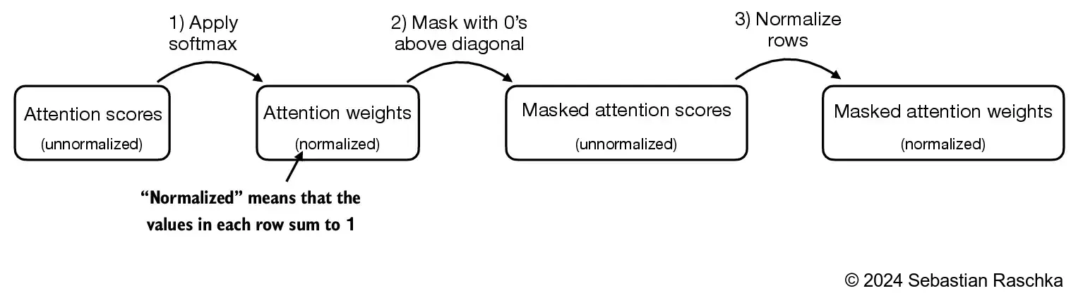
masked_simple = attn_weights*mask_simple
print(masked_simple)
tensor([[0.1921, 0.0000, 0.0000, 0.0000, 0.0000, 0.0000],
[0.2041, 0.1659, 0.0000, 0.0000, 0.0000, 0.0000],
[0.2036, 0.1659, 0.1662, 0.0000, 0.0000, 0.0000],
[0.1869, 0.1667, 0.1668, 0.1571, 0.0000, 0.0000],
[0.1830, 0.1669, 0.1670, 0.1588, 0.1658, 0.0000],
[0.1935, 0.1663, 0.1666, 0.1542, 0.1666, 0.1529]],
grad_fn=<MulBackward0>)In [28]:
row_sums = masked_simple.sum(dim=-1, keepdim=True)
masked_simple_norm = masked_simple / row_sums
print(masked_simple_norm)
tensor([[1.0000, 0.0000, 0.0000, 0.0000, 0.0000, 0.0000],
[0.5517, 0.4483, 0.0000, 0.0000, 0.0000, 0.0000],
[0.3800, 0.3097, 0.3103, 0.0000, 0.0000, 0.0000],
[0.2758, 0.2460, 0.2462, 0.2319, 0.0000, 0.0000],
[0.2175, 0.1983, 0.1984, 0.1888, 0.1971, 0.0000],
[0.1935, 0.1663, 0.1666, 0.1542, 0.1666, 0.1529]],
grad_fn=<DivBackward0>)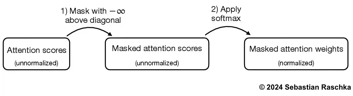
In [29]:
mask = torch.triu(torch.ones(context_length, context_length), diagonal=1)
masked = attn_scores.masked_fill(mask.bool(), -torch.inf)
print(masked)
tensor([[0.2899, -inf, -inf, -inf, -inf, -inf],
[0.4656, 0.1723, -inf, -inf, -inf, -inf],
[0.4594, 0.1703, 0.1731, -inf, -inf, -inf],
[0.2642, 0.1024, 0.1036, 0.0186, -inf, -inf],
[0.2183, 0.0874, 0.0882, 0.0177, 0.0786, -inf],
[0.3408, 0.1270, 0.1290, 0.0198, 0.1290, 0.0078]],
grad_fn=<MaskedFillBackward0>)In [30]:
attn_weights = torch.softmax(masked / keys.shape[-1]**0.5, dim=-1)
print(attn_weights)
tensor([[1.0000, 0.0000, 0.0000, 0.0000, 0.0000, 0.0000],
[0.5517, 0.4483, 0.0000, 0.0000, 0.0000, 0.0000],
[0.3800, 0.3097, 0.3103, 0.0000, 0.0000, 0.0000],
[0.2758, 0.2460, 0.2462, 0.2319, 0.0000, 0.0000],
[0.2175, 0.1983, 0.1984, 0.1888, 0.1971, 0.0000],
[0.1935, 0.1663, 0.1666, 0.1542, 0.1666, 0.1529]],
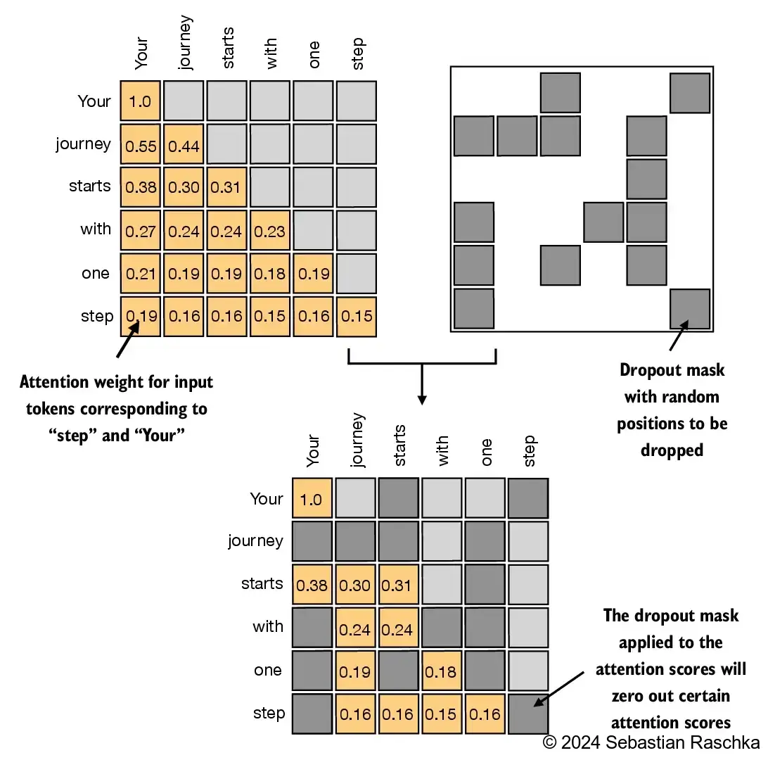
grad_fn=<SoftmaxBackward0>)In addition, we also apply dropout to reduce overfitting during training
Dropout can be applied in several places:
Here, we will apply the dropout mask after computing the attention weights because it’s more common
Furthermore, in this specific example, we use a dropout rate of 50%, which means randomly masking out half of the attention weights. (When we train the GPT model later, we will use a lower dropout rate, such as 0.1 or 0.2
dropout_rate)In [31]:
torch.manual_seed(123)
dropout = torch.nn.Dropout(0.5) # dropout rate of 50%
example = torch.ones(6, 6) # create a matrix of ones

print(dropout(example))
tensor([[2., 2., 0., 2., 2., 0.],
[0., 0., 0., 2., 0., 2.],
[2., 2., 2., 2., 0., 2.],
[0., 2., 2., 0., 0., 2.],
[0., 2., 0., 2., 0., 2.],
[0., 2., 2., 2., 2., 0.]])In [32]:
torch.manual_seed(123)
print(dropout(attn_weights))
tensor([[2.0000, 0.0000, 0.0000, 0.0000, 0.0000, 0.0000],
[0.0000, 0.0000, 0.0000, 0.0000, 0.0000, 0.0000],
[0.7599, 0.6194, 0.6206, 0.0000, 0.0000, 0.0000],
[0.0000, 0.4921, 0.4925, 0.0000, 0.0000, 0.0000],
[0.0000, 0.3966, 0.0000, 0.3775, 0.0000, 0.0000],
[0.0000, 0.3327, 0.3331, 0.3084, 0.3331, 0.0000]],
grad_fn=<MulBackward0>)CausalAttention class supports the batch outputs produced by the data loader we implemented in chapter 2In [33]:
batch = torch.stack((inputs, inputs), dim=0)
print(batch.shape) # 2 inputs with 6 tokens each, and each token has embedding dimension 3
torch.Size([2, 6, 3])In [34]:
class CausalAttention(nn.Module):

    def __init__(self, d_in, d_out, context_length,
                 dropout, qkv_bias=False):
        super().__init__()
        self.d_out = d_out
        self.W_query = nn.Linear(d_in, d_out, bias=qkv_bias)
        self.W_key   = nn.Linear(d_in, d_out, bias=qkv_bias)
        self.W_value = nn.Linear(d_in, d_out, bias=qkv_bias)
        self.dropout = nn.Dropout(dropout) # New
        self.register_buffer('mask', torch.triu(torch.ones(context_length, context_length), diagonal=1)) # New

    def forward(self, x):
        b, num_tokens, d_in = x.shape # New batch dimension b
        # For inputs where `num_tokens` exceeds `context_length`, this will result in errors
        # in the mask creation further below.
        # In practice, this is not a problem since the LLM (chapters 4-7) ensures that inputs
        # do not exceed `context_length` before reaching this forward method.
        keys = self.W_key(x)
        queries = self.W_query(x)
        values = self.W_value(x)

        attn_scores = queries @ keys.transpose(1, 2) # Changed transpose
        attn_scores.masked_fill_(  # New, _ ops are in-place
            self.mask.bool()[:num_tokens, :num_tokens], -torch.inf)  # `:num_tokens` to account for cases where the number of tokens in the batch is smaller than the supported context_size
        attn_weights = torch.softmax(
            attn_scores / keys.shape[-1]**0.5, dim=-1
        )
        attn_weights = self.dropout(attn_weights) # New

        context_vec = attn_weights @ values
        return context_vec

torch.manual_seed(123)

context_length = batch.shape[1]
ca = CausalAttention(d_in, d_out, context_length, 0.0)

context_vecs = ca(batch)

print(context_vecs)
print("context_vecs.shape:", context_vecs.shape)
tensor([[[-0.4519, 0.2216],
[-0.5874, 0.0058],
[-0.6300, -0.0632],
[-0.5675, -0.0843],
[-0.5526, -0.0981],
[-0.5299, -0.1081]],
[[-0.4519, 0.2216],
[-0.5874, 0.0058],
[-0.6300, -0.0632],
[-0.5675, -0.0843],
[-0.5526, -0.0981],
[-0.5299, -0.1081]]], grad_fn=<UnsafeViewBackward0>)
context_vecs.shape: torch.Size([2, 6, 2])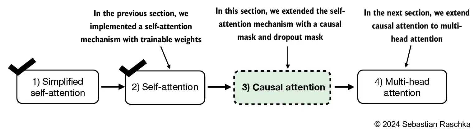
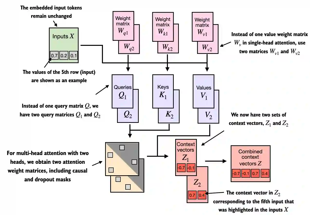
Below is a summary of the self-attention implemented previously (causal and dropout masks not shown for simplicity)
This is also called single-head attention:
In [35]:
class MultiHeadAttentionWrapper(nn.Module):

    def __init__(self, d_in, d_out, context_length, dropout, num_heads, qkv_bias=False):
        super().__init__()
        self.heads = nn.ModuleList(
            [CausalAttention(d_in, d_out, context_length, dropout, qkv_bias)
             for _ in range(num_heads)]
        )

    def forward(self, x):
        return torch.cat([head(x) for head in self.heads], dim=-1)


torch.manual_seed(123)

context_length = batch.shape[1] # This is the number of tokens
d_in, d_out = 3, 2
mha = MultiHeadAttentionWrapper(
    d_in, d_out, context_length, 0.0, num_heads=2
)

context_vecs = mha(batch)

print(context_vecs)
print("context_vecs.shape:", context_vecs.shape)
tensor([[[-0.4519, 0.2216, 0.4772, 0.1063],
[-0.5874, 0.0058, 0.5891, 0.3257],
[-0.6300, -0.0632, 0.6202, 0.3860],
[-0.5675, -0.0843, 0.5478, 0.3589],
[-0.5526, -0.0981, 0.5321, 0.3428],
[-0.5299, -0.1081, 0.5077, 0.3493]],
[[-0.4519, 0.2216, 0.4772, 0.1063],
[-0.5874, 0.0058, 0.5891, 0.3257],
[-0.6300, -0.0632, 0.6202, 0.3860],
[-0.5675, -0.0843, 0.5478, 0.3589],
[-0.5526, -0.0981, 0.5321, 0.3428],
[-0.5299, -0.1081, 0.5077, 0.3493]]], grad_fn=<CatBackward0>)
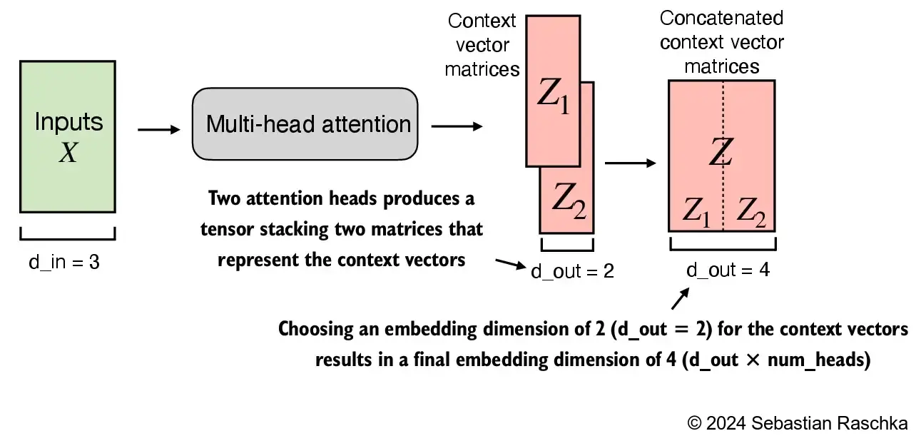
context_vecs.shape: torch.Size([2, 6, 4])d_out=2 as the embedding dimension for the key, query, and value vectors as well as the context vector. And since we have 2 attention heads, we have the output embedding dimension 2*2=4While the above is an intuitive and fully functional implementation of multi-head attention (wrapping the single-head attention CausalAttention implementation from earlier), we can write a stand-alone class called MultiHeadAttention to achieve the same
We don’t concatenate single attention heads for this stand-alone MultiHeadAttention class
Instead, we create single W_query, W_key, and W_value weight matrices and then split those into individual matrices for each attention head:
In [36]:
class MultiHeadAttention(nn.Module):
    def __init__(self, d_in, d_out, context_length, dropout, num_heads, qkv_bias=False):
        super().__init__()
        assert (d_out % num_heads == 0), \
            "d_out must be divisible by num_heads"

        self.d_out = d_out
        self.num_heads = num_heads
        self.head_dim = d_out // num_heads # Reduce the projection dim to match desired output dim

        self.W_query = nn.Linear(d_in, d_out, bias=qkv_bias)
        self.W_key = nn.Linear(d_in, d_out, bias=qkv_bias)
        self.W_value = nn.Linear(d_in, d_out, bias=qkv_bias)
        self.out_proj = nn.Linear(d_out, d_out)  # Linear layer to combine head outputs
        self.dropout = nn.Dropout(dropout)
        self.register_buffer(
            "mask",
            torch.triu(torch.ones(context_length, context_length),
                       diagonal=1)
        )

    def forward(self, x):
        b, num_tokens, d_in = x.shape
        # As in `CausalAttention`, for inputs where `num_tokens` exceeds `context_length`,
        # this will result in errors in the mask creation further below.
        # In practice, this is not a problem since the LLM (chapters 4-7) ensures that inputs
        # do not exceed `context_length` before reaching this forwar

        keys = self.W_key(x) # Shape: (b, num_tokens, d_out)
        queries = self.W_query(x)
        values = self.W_value(x)

        # We implicitly split the matrix by adding a `num_heads` dimension
        # Unroll last dim: (b, num_tokens, d_out) -> (b, num_tokens, num_heads, head_dim)
        keys = keys.view(b, num_tokens, self.num_heads, self.head_dim)
        values = values.view(b, num_tokens, self.num_heads, self.head_dim)
        queries = queries.view(b, num_tokens, self.num_heads, self.head_dim)

        # Transpose: (b, num_tokens, num_heads, head_dim) -> (b, num_heads, num_tokens, head_dim)
        keys = keys.transpose(1, 2)
        queries = queries.transpose(1, 2)
        values = values.transpose(1, 2)

        # Compute scaled dot-product attention (aka self-attention) with a causal mask
        attn_scores = queries @ keys.transpose(2, 3)  # Dot product for each head

        # Original mask truncated to the number of tokens and converted to boolean
        mask_bool = self.mask.bool()[:num_tokens, :num_tokens]

        # Use the mask to fill attention scores
        attn_scores.masked_fill_(mask_bool, -torch.inf)

        attn_weights = torch.softmax(attn_scores / keys.shape[-1]**0.5, dim=-1)
        attn_weights = self.dropout(attn_weights)

        # Shape: (b, num_tokens, num_heads, head_dim)
        context_vec = (attn_weights @ values).transpose(1, 2)

        # Combine heads, where self.d_out = self.num_heads * self.head_dim
        context_vec = context_vec.contiguous().view(b, num_tokens, self.d_out)
        context_vec = self.out_proj(context_vec) # optional projection

        return context_vec

torch.manual_seed(123)

batch_size, context_length, d_in = batch.shape
d_out = 2
mha = MultiHeadAttention(d_in, d_out, context_length, 0.0, num_heads=2)

context_vecs = mha(batch)

print(context_vecs)
print("context_vecs.shape:", context_vecs.shape)
tensor([[[0.3190, 0.4858],
[0.2943, 0.3897],
[0.2856, 0.3593],
[0.2693, 0.3873],
[0.2639, 0.3928],
[0.2575, 0.4028]],
[[0.3190, 0.4858],
[0.2943, 0.3897],
[0.2856, 0.3593],
[0.2693, 0.3873],
[0.2639, 0.3928],
[0.2575, 0.4028]]], grad_fn=<ViewBackward0>)
context_vecs.shape: torch.Size([2, 6, 2])MultiHeadAttentionWrapper that is more efficientself.out_proj) to the MultiHeadAttention class above. This is simply a linear transformation that doesn’t change the dimensions. It’s a standard convention to use such a projection layer in LLM implementation, but it’s not strictly necessary (recent research has shown that it can be removed without affecting the modeling performance; see the further reading section at the end of this chapter)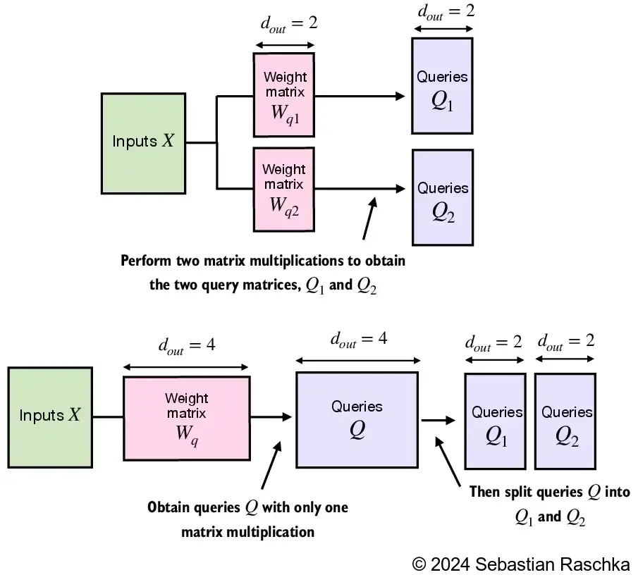
torch.nn.MultiheadAttention class in PyTorchattn_scores = queries @ keys.transpose(2, 3):In [37]:
# (b, num_heads, num_tokens, head_dim) = (1, 2, 3, 4)
a = torch.tensor([[[[0.2745, 0.6584, 0.2775, 0.8573],
                    [0.8993, 0.0390, 0.9268, 0.7388],
                    [0.7179, 0.7058, 0.9156, 0.4340]],

                   [[0.0772, 0.3565, 0.1479, 0.5331],
                    [0.4066, 0.2318, 0.4545, 0.9737],
                    [0.4606, 0.5159, 0.4220, 0.5786]]]])

print(a @ a.transpose(2, 3))
tensor([[[[1.3208, 1.1631, 1.2879],
[1.1631, 2.2150, 1.8424],
[1.2879, 1.8424, 2.0402]],
[[0.4391, 0.7003, 0.5903],
[0.7003, 1.3737, 1.0620],
[0.5903, 1.0620, 0.9912]]]])In this case, the matrix multiplication implementation in PyTorch will handle the 4-dimensional input tensor so that the matrix multiplication is carried out between the 2 last dimensions (num_tokens, head_dim) and then repeated for the individual heads
For instance, the following becomes a more compact way to compute the matrix multiplication for each head separately:
In [38]:
first_head = a[0, 0, :, :]
first_res = first_head @ first_head.T
print("First head:\n", first_res)

second_head = a[0, 1, :, :]
second_res = second_head @ second_head.T
print("\nSecond head:\n", second_res)
First head:
tensor([[1.3208, 1.1631, 1.2879],
[1.1631, 2.2150, 1.8424],
[1.2879, 1.8424, 2.0402]])
Second head:
tensor([[0.4391, 0.7003, 0.5903],
[0.7003, 1.3737, 1.0620],
[0.5903, 1.0620, 0.9912]])